Note
Go to the end to download the full example code.
PSF model usage in ctapipe#
 7 import astropy.units as u
 8 import numpy as np
 9 from itertools import product
10 from ctapipe.instrument.optics import ComaPSFModel
11 from ctapipe.instrument import SubarrayDescription
12 import matplotlib.pyplot as plt
13
14 # %matplotlib inline
15
16
17 # make plots and fonts larger
18 plt.rcParams["figure.figsize"] = (12, 8)
19 plt.rcParams["font.size"] = 16
Set up the PSF model#
This sets up the PSF model describing pure coma aberrations PSF effect for the LSTs. The parameters are taken from [A+23], which was original given in polar coordinates in the camera frame. We here manually convert the parameters using the plate scale of LSTs to get the parameters in the TelescopeFrame.
36 subarray = SubarrayDescription.read("dataset://gamma_prod5.simtel.zst")
37
38 lst_plate_scale_deg = np.rad2deg(
39     1.0 / subarray.tel[1].optics.effective_focal_length.to_value(u.m)
40 )
41
42 lst1 = subarray.select_subarray([1])
43
44 psf_model = ComaPSFModel(
45     subarray=lst1,
46     asymmetry_max=0.49244797,
47     asymmetry_decay_rate=9.23573115 / lst_plate_scale_deg,
48     asymmetry_linear_term=0.15216096 / lst_plate_scale_deg,
49     radial_scale_offset=0.01409259 * lst_plate_scale_deg,
50     radial_scale_linear=0.02947208,
51     radial_scale_quadratic=0.06000271 / lst_plate_scale_deg**1,
52     radial_scale_cubic=-0.02969355 / lst_plate_scale_deg**2,
53     polar_scale_amplitude=0.24271557,
54     polar_scale_decay=7.5511501 / lst_plate_scale_deg,
55     polar_scale_offset=0.02037972 * lst_plate_scale_deg,
56 )
calculate PSF at different positions in the field of view
64 lon0 = 1 * lst_plate_scale_deg * u.deg
65 lat0 = 1 * lst_plate_scale_deg * u.deg
66
67 edges_x = (
68     np.linspace(-0.1 * lst_plate_scale_deg, 0.1 * lst_plate_scale_deg, 250) * u.deg
69 )
70 edges_y = (
71     np.linspace(-0.1 * lst_plate_scale_deg, 0.1 * lst_plate_scale_deg, 250) * u.deg
72 )
73 centers_x = 0.5 * (edges_x[:-1] + edges_x[1:])
74 centers_y = 0.5 * (edges_y[:-1] + edges_y[1:])
75 x, y = np.meshgrid(centers_x, centers_y)
76
77 psf_center = psf_model.pdf(tel_id=1, lon=x, lat=y, lon0=0.0 * u.deg, lat0=0.0 * u.deg)
78 psf_border = psf_model.pdf(
79     tel_id=1,
80     lon=x + 1 * lst_plate_scale_deg * u.deg,
81     lat=y + 1 * lst_plate_scale_deg * u.deg,
82     lon0=lon0,
83     lat0=lat0,
84 )
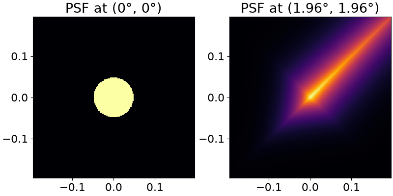
Plot the results#
 92 fig, (ax1, ax2) = plt.subplots(1, 2, layout="constrained", figsize=(8, 4))
 93
 94 ax1.pcolormesh(
 95     edges_x.to_value(u.deg),
 96     edges_y.to_value(u.deg),
 97     psf_center,
 98     cmap="inferno",
 99 )
100
101 ax2.pcolormesh(
102     edges_x.to_value(u.deg),
103     edges_y.to_value(u.deg),
104     psf_border,
105     cmap="inferno",
106 )
107
108 ax1.set(
109     aspect=1,
110     title="PSF at (0°, 0°)",
111 )
112 ax2.set(
113     aspect=1,
114     title=f"PSF at ({lon0.to_value(u.deg):.2f}°, {lat0.to_value(u.deg):.2f}°)",
115 )
116 plt.show()
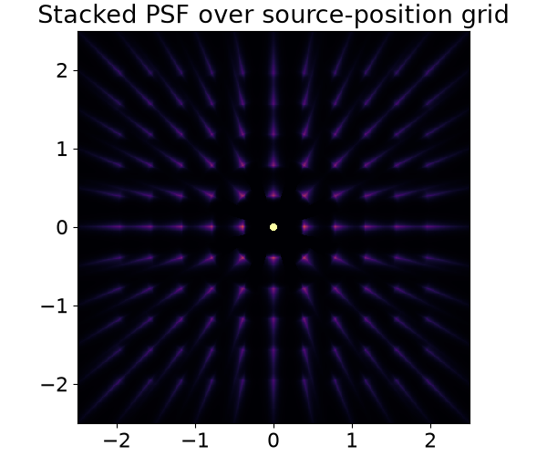
Stacked PSF over multiple source positions#
124 lons = np.linspace(-1.0, 1.0, 11) * lst_plate_scale_deg * u.deg
125 lats = np.linspace(-1.0, 1.0, 11) * lst_plate_scale_deg * u.deg
126
127 edges_x_stack = np.linspace(-2.5 * u.deg, 2.5 * u.deg, 500)
128 edges_y_stack = np.linspace(-2.5 * u.deg, 2.5 * u.deg, 500)
129 centers_x_stack = 0.5 * (edges_x_stack[:-1] + edges_x_stack[1:])
130 centers_y_stack = 0.5 * (edges_y_stack[:-1] + edges_y_stack[1:])
131 x_stack, y_stack = np.meshgrid(centers_x_stack, centers_y_stack)
132
133 psf_stacked = np.zeros(x_stack.shape)
134 for source_lon, source_lat in product(lons, lats):
135     psf_stacked += psf_model.pdf(
136         tel_id=1,
137         lon=x_stack,
138         lat=y_stack,
139         lon0=source_lon,
140         lat0=source_lat,
141     )
142
143 fig_stack, ax_stack = plt.subplots(1, 1, layout="constrained", figsize=(6, 5))
144 mesh = ax_stack.pcolormesh(
145     edges_x_stack.to_value(u.deg),
146     edges_y_stack.to_value(u.deg),
147     psf_stacked,
148     cmap="inferno",
149 )
150 ax_stack.set(aspect=1, title="Stacked PSF over source-position grid")
151 plt.show()
Total running time of the script: (0 minutes 3.353 seconds)