Analyzing Events Using ctapipe

Initially presented @ LST Analysis Bootcamp in Padova, 26.11.2018 by Maximilian Nöthe (@maxnoe) & Kai A. Brügge (@mackaiver)

import tempfile
import timeit
from copy import deepcopy

import astropy.units as u
import matplotlib.pyplot as plt
import numpy as np
from astropy.coordinates import AltAz, angular_separation
from matplotlib.colors import ListedColormap
from scipy.sparse.csgraph import connected_components
from traitlets.config import Config

from ctapipe.calib import CameraCalibrator
from ctapipe.image import (
    ImageProcessor,
    camera_to_shower_coordinates,
    concentration_parameters,
    hillas_parameters,
    leakage_parameters,
    number_of_islands,
    timing_parameters,
    toymodel,
)
from ctapipe.image.cleaning import tailcuts_clean
from ctapipe.io import DataWriter, EventSource, TableLoader
from ctapipe.reco import ShowerProcessor
from ctapipe.utils.datasets import get_dataset_path
from ctapipe.visualization import ArrayDisplay, CameraDisplay

# %matplotlib inline

plt.rcParams["figure.figsize"] = (12, 8)
plt.rcParams["font.size"] = 14
plt.rcParams["figure.figsize"]

[12.0, 8.0]

General Information

Design

• DL0 → DL3 analysis

• Currently some R0 → DL2 code to be able to analyze simtel files

• ctapipe is built upon the Scientific Python Stack, core dependencies are

  • numpy

  • scipy

  • astropy

  • numba

Development

• ctapipe is developed as Open Source Software (BSD 3-Clause License) at cta-observatory/ctapipe

• We use the “Github-Workflow”:

  • Few people (e.g. @kosack, @maxnoe) have write access to the main repository

  • Contributors fork the main repository and work on branches

  • Pull Requests are merged after Code Review and automatic execution of the test suite

• Early development stage ⇒ backwards-incompatible API changes might and will happen

What’s there?

• Reading simtel simulation files

• Simple calibration, cleaning and feature extraction functions

• Camera and Array plotting

• Coordinate frames and transformations

• Stereo-reconstruction using line intersections

What’s still missing?

• Good integration with machine learning techniques

• IRF calculation

• Documentation, e.g. formal definitions of coordinate frames

What can you do?

• Report issues

  • Hard to get started? Tell us where you are stuck

  • Tell user stories

  • Missing features

• Start contributing

  • ctapipe needs more workpower

  • Implement new reconstruction features

A simple hillas analysis

Reading in simtel files

input_url = get_dataset_path("gamma_prod5.simtel.zst")

# EventSource() automatically detects what kind of file we are giving it,
# if already supported by ctapipe
source = EventSource(input_url, max_events=5)

print(type(source))

<class 'ctapipe.io.simteleventsource.SimTelEventSource'>

for event in source:
    print(
        "Id: {}, E = {:1.3f}, Telescopes: {}".format(
            event.count, event.simulation.shower.energy, len(event.r0.tel)
        )
    )

Id: 0, E = 0.073 TeV, Telescopes: 3
Id: 1, E = 1.745 TeV, Telescopes: 14
Id: 2, E = 1.745 TeV, Telescopes: 4
Id: 3, E = 1.745 TeV, Telescopes: 20
Id: 4, E = 1.745 TeV, Telescopes: 31

Each event is a DataContainer holding several Fields of data, which can be containers or just numbers. Let’s look a one event:

event

ctapipe.containers.ArrayEventContainer:
                       index.*: event indexing information with default None
                          r0.*: Raw Data with default None
                          r1.*: R1 Calibrated Data with default None
                         dl0.*: DL0 Data Volume Reduced Data with default None
                         dl1.*: DL1 Calibrated image with default None
                         dl2.*: DL2 reconstruction info with default None
                  simulation.*: Simulated Event Information with default None
                                with type <class
                                'ctapipe.containers.SimulatedEventContainer'>
                     trigger.*: central trigger information with default None
                         count: number of events processed with default 0
                  monitoring.*: container for event-wise monitoring data (MON)
                                with default None
                        muon.*: Container for muon analysis results with default
                                None

source.subarray.camera_types

(CameraDescription(name=CHEC, geometry=CHEC, readout=CHEC), CameraDescription(name=FlashCam, geometry=FlashCam, readout=FlashCam), CameraDescription(name=LSTCam, geometry=LSTCam, readout=LSTCam), CameraDescription(name=NectarCam, geometry=NectarCam, readout=NectarCam))

len(event.r0.tel), len(event.r1.tel)

(31, 31)

Data calibration

The CameraCalibrator calibrates the event (obtaining the dl1 images).

calibrator = CameraCalibrator(subarray=source.subarray)

calibrator(event)

Event displays

Let’s use ctapipe’s plotting facilities to plot the telescope images

event.dl1.tel.keys()

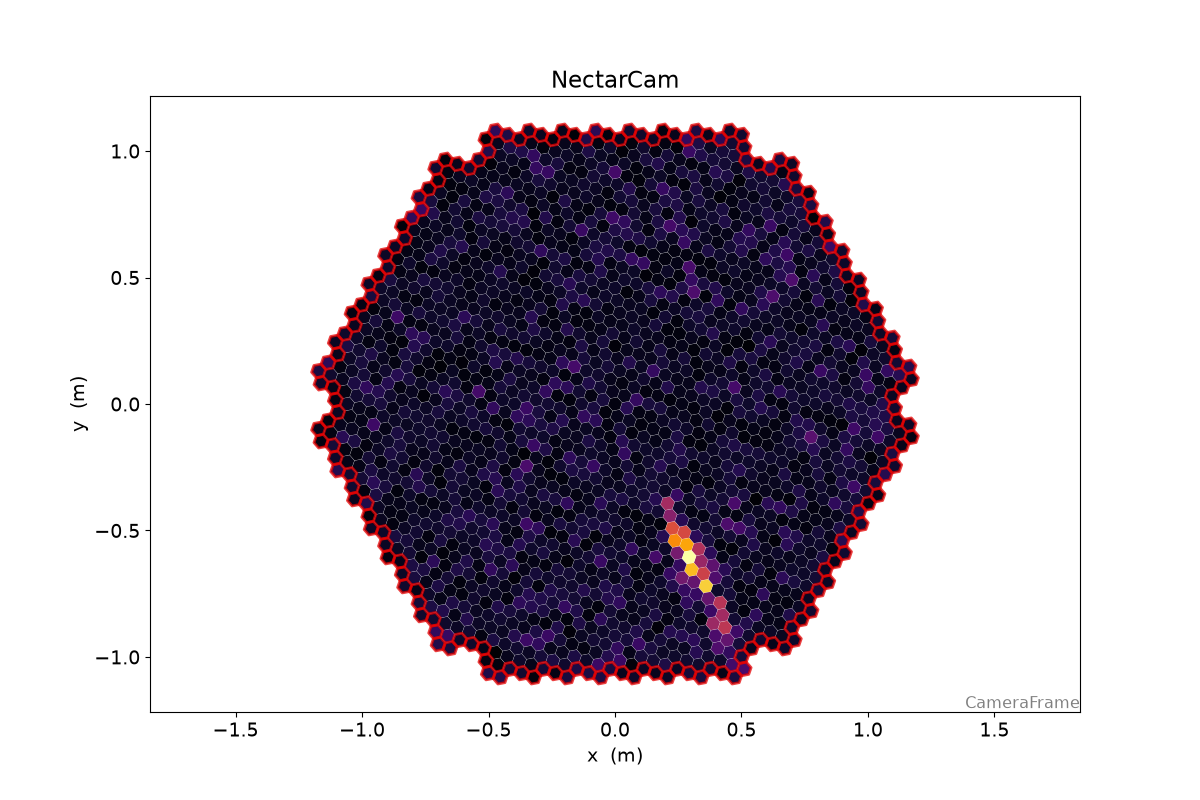
dict_keys([3, 4, 8, 9, 14, 15, 23, 24, 25, 29, 32, 36, 42, 46, 52, 56, 103, 104, 109, 110, 118, 119, 120, 126, 127, 129, 130, 137, 139, 143, 161])

tel_id = 130

geometry = source.subarray.tel[tel_id].camera.geometry
dl1 = event.dl1.tel[tel_id]

geometry, dl1

(CameraGeometry(name='NectarCam', pix_type=PixelShape.HEXAGON, npix=1855, cam_rot=0.000 deg, pix_rot=40.893 deg, frame=<CameraFrame Frame (focal_length=16.445049285888672 m, rotation=0.0 rad, telescope_pointing=None, obstime=None, location=None)>), ctapipe.containers.DL1CameraContainer:
                         image: Numpy array of camera image, after waveform
                                extraction.Shape: (n_pixel) if n_channels is 1
                                or data is gain selectedelse: (n_channels,
                                n_pixel) with default None
                     peak_time: Numpy array containing position of the peak of
                                the pulse as determined by the extractor.Shape:
                                (n_pixel) if n_channels is 1 or data is gain
                                selectedelse: (n_channels, n_pixel) with default
                                None
                    image_mask: Boolean numpy array where True means the pixel
                                has passed cleaning. Shape: (n_pixel, ) with
                                default None as a 1-D array with dtype bool
                      is_valid: True if image extraction succeeded, False if
                                failed or in the case of TwoPass methods, that
                                the first pass only was returned. with default
                                False
                    parameters: Image parameters with default None with type
                                <class
                                'ctapipe.containers.ImageParametersContainer'>)

dl1.image

array([-0.3856395 ,  1.2851689 ,  1.403967  , ...,  2.6847053 ,
        0.04941979, -1.0566036 ], shape=(1855,), dtype=float32)

display = CameraDisplay(geometry)

# right now, there might be one image per gain channel.
# This will change as soon as
display.image = dl1.image
display.add_colorbar()

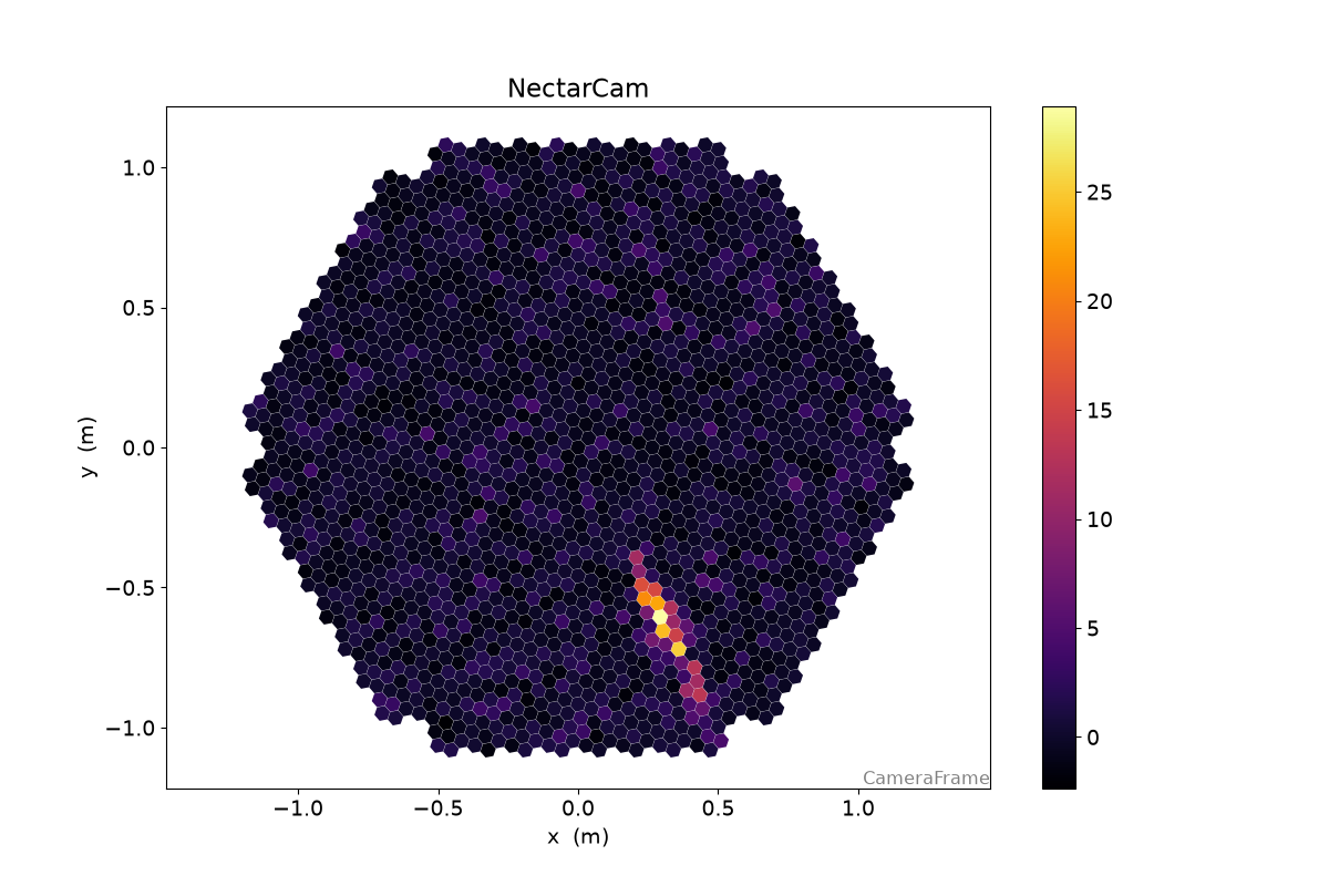
Image Cleaning

# unoptimized cleaning levels
cleaning_level = {
    "CHEC": (2, 4, 2),
    "LSTCam": (3.5, 7, 2),
    "FlashCam": (3.5, 7, 2),
    "NectarCam": (4, 8, 2),
}

boundary, picture, min_neighbors = cleaning_level[geometry.name]

clean = tailcuts_clean(
    geometry,
    dl1.image,
    boundary_thresh=boundary,
    picture_thresh=picture,
    min_number_picture_neighbors=min_neighbors,
)

fig, (ax1, ax2) = plt.subplots(1, 2, figsize=(15, 5))

d1 = CameraDisplay(geometry, ax=ax1)
d2 = CameraDisplay(geometry, ax=ax2)

ax1.set_title("Image")
d1.image = dl1.image
d1.add_colorbar(ax=ax1)

ax2.set_title("Pulse Time")
d2.image = dl1.peak_time - np.average(dl1.peak_time, weights=dl1.image)
d2.cmap = "RdBu_r"
d2.add_colorbar(ax=ax2)
d2.set_limits_minmax(-20, 20)

d1.highlight_pixels(clean, color="red", linewidth=1)

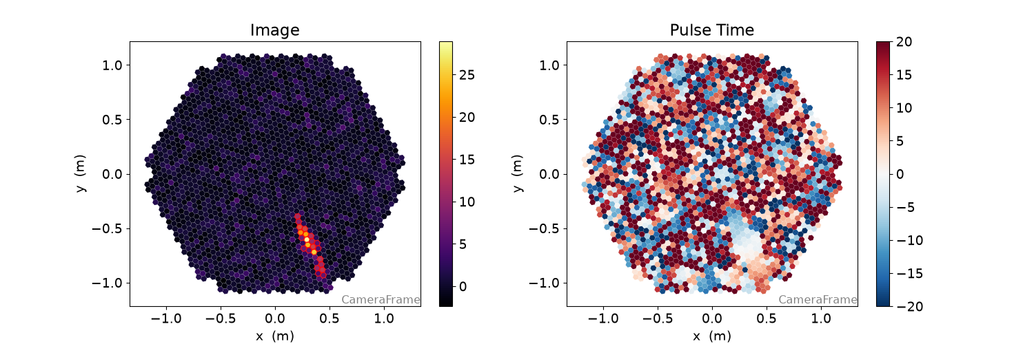
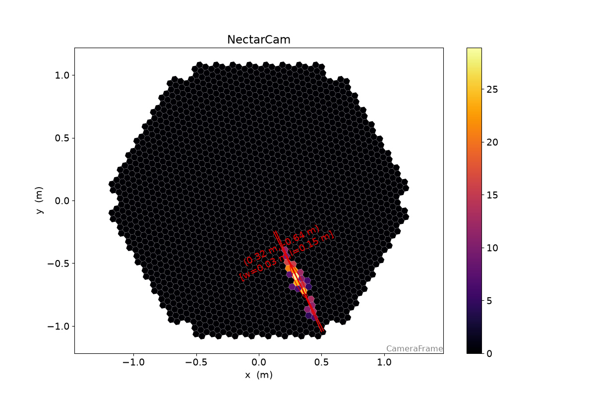
Image Parameters

hillas = hillas_parameters(geometry[clean], dl1.image[clean])

print(hillas)

{'intensity': np.float64(303.9444303512573),
 'kurtosis': np.float64(2.4649477808816265),
 'length': <Quantity 0.14667835 m>,
 'length_uncertainty': <Quantity 0.00509155 m>,
 'phi': <Angle -1.11344351 rad>,
 'psi': <Angle -1.12308339 rad>,
 'psi_uncertainty': <Angle 0.01927114 rad>,
 'r': <Quantity 0.71788425 m>,
 'skewness': np.float64(0.360906379879541),
 'transverse_cog_uncertainty': <Quantity 0.00261556 m>,
 'width': <Quantity 0.02584731 m>,
 'width_uncertainty': <Quantity 0.00111159 m>,
 'x': <Quantity 0.31699941 m>,
 'y': <Quantity -0.64410339 m>}

display = CameraDisplay(geometry)

# set "unclean" pixels to 0
cleaned = dl1.image.copy()
cleaned[~clean] = 0.0

display.image = cleaned
display.add_colorbar()

display.overlay_moments(hillas, color="xkcd:red")

timing = timing_parameters(geometry, dl1.image, dl1.peak_time, hillas, clean)

print(timing)

{'deviation': 0.792151827050336,
 'intercept': np.float64(21.81257256241495),
 'slope': <Quantity 31.32320575 1 / m>}

long, trans = camera_to_shower_coordinates(
    geometry.pix_x, geometry.pix_y, hillas.x, hillas.y, hillas.psi
)

plt.plot(long[clean], dl1.peak_time[clean], "o")
plt.plot(long[clean], timing.slope * long[clean] + timing.intercept)

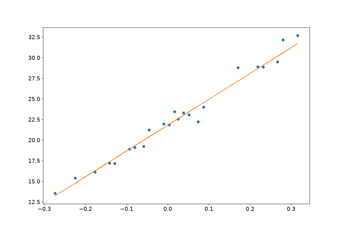
[<matplotlib.lines.Line2D object at 0x7c2220192960>]

leakage = leakage_parameters(geometry, dl1.image, clean)
print(leakage)

{'intensity_width_1': np.float32(0.0),
 'intensity_width_2': np.float32(0.0),
 'pixels_width_1': np.float64(0.0),
 'pixels_width_2': np.float64(0.0)}

disp = CameraDisplay(geometry)
disp.image = dl1.image
disp.highlight_pixels(geometry.get_border_pixel_mask(1), linewidth=2, color="xkcd:red")

n_islands, island_id = number_of_islands(geometry, clean)

print(n_islands)

2

conc = concentration_parameters(geometry, dl1.image, hillas)
print(conc)

{'cog': np.float64(0.2571728392782083),
 'core': np.float64(0.4014042974365615),
 'pixel': np.float64(0.09514053791448862)}

Putting it all together / Stereo reconstruction

All these steps are now unified in several components configurable through the config system, mainly:

• CameraCalibrator for DL0 → DL1 (Images)

• ImageProcessor for DL1 (Images) → DL1 (Parameters)

• ShowerProcessor for stereo reconstruction of the shower geometry

• DataWriter for writing data into HDF5

A command line tool doing these steps and writing out data in HDF5 format is available as ctapipe-process

image_processor_config = Config(
    {
        "ImageProcessor": {
            "image_cleaner_type": "TailcutsImageCleaner",
            "TailcutsImageCleaner": {
                "picture_threshold_pe": [
                    ("type", "LST_LST_LSTCam", 7.5),
                    ("type", "MST_MST_FlashCam", 8),
                    ("type", "MST_MST_NectarCam", 8),
                    ("type", "SST_ASTRI_CHEC", 7),
                ],
                "boundary_threshold_pe": [
                    ("type", "LST_LST_LSTCam", 5),
                    ("type", "MST_MST_FlashCam", 4),
                    ("type", "MST_MST_NectarCam", 4),
                    ("type", "SST_ASTRI_CHEC", 4),
                ],
            },
        }
    }
)

input_url = get_dataset_path("gamma_prod5.simtel.zst")
source = EventSource(input_url)

calibrator = CameraCalibrator(subarray=source.subarray)
image_processor = ImageProcessor(
    subarray=source.subarray, config=image_processor_config
)
shower_processor = ShowerProcessor(subarray=source.subarray)
horizon_frame = AltAz()

f = tempfile.NamedTemporaryFile(suffix=".hdf5")

with DataWriter(source, output_path=f.name, overwrite=True, write_dl2=True) as writer:
    for event in source:
        energy = event.simulation.shower.energy
        n_telescopes_r1 = len(event.r1.tel)
        event_id = event.index.event_id
        print(f"Id: {event_id}, E = {energy:1.3f}, Telescopes (R1): {n_telescopes_r1}")

        calibrator(event)
        image_processor(event)
        shower_processor(event)

        stereo = event.dl2.stereo.geometry["HillasReconstructor"]
        if stereo.is_valid:
            print("  Alt: {:.2f}°".format(stereo.alt.deg))
            print("  Az: {:.2f}°".format(stereo.az.deg))
            print("  Hmax: {:.0f}".format(stereo.h_max))
            print("  CoreX: {:.1f}".format(stereo.core_x))
            print("  CoreY: {:.1f}".format(stereo.core_y))
            print("  Multiplicity: {:d}".format(len(stereo.telescopes)))

        # save a nice event for plotting later
        if event.count == 3:
            plotting_event = deepcopy(event)

        writer(event)

Overwriting /tmp/tmpxlmq768m.hdf5
Id: 4009, E = 0.073 TeV, Telescopes (R1): 3
  Alt: 70.18°
  Az: 0.41°
  Hmax: 14066 m
  CoreX: -113.2 m
  CoreY: 366.5 m
  Multiplicity: 3
Id: 5101, E = 1.745 TeV, Telescopes (R1): 14
  Alt: 70.00°
  Az: 359.95°
  Hmax: 10329 m
  CoreX: -739.5 m
  CoreY: -268.4 m
  Multiplicity: 10
Id: 5103, E = 1.745 TeV, Telescopes (R1): 4
  Alt: 70.21°
  Az: 0.50°
  Hmax: 11526 m
  CoreX: 832.1 m
  CoreY: 945.4 m
  Multiplicity: 2
Id: 5104, E = 1.745 TeV, Telescopes (R1): 20
  Alt: 70.16°
  Az: 0.07°
  Hmax: 10643 m
  CoreX: -518.3 m
  CoreY: -451.5 m
  Multiplicity: 15
Id: 5105, E = 1.745 TeV, Telescopes (R1): 31
  Alt: 70.02°
  Az: 0.13°
  Hmax: 10449 m
  CoreX: -327.7 m
  CoreY: 408.8 m
  Multiplicity: 25
Id: 5108, E = 1.745 TeV, Telescopes (R1): 3
  Alt: 69.95°
  Az: 359.79°
  Hmax: 10409 m
  CoreX: -1304.5 m
  CoreY: 205.6 m
  Multiplicity: 2
Id: 5109, E = 1.745 TeV, Telescopes (R1): 8
  Alt: 69.62°
  Az: 359.93°
  Hmax: 10886 m
  CoreX: -1067.6 m
  CoreY: 480.5 m
  Multiplicity: 3

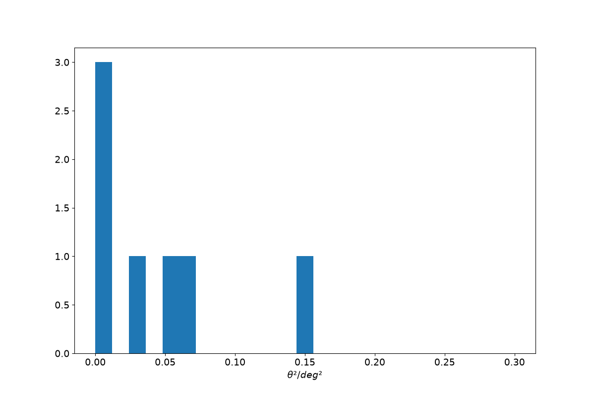
loader = TableLoader(f.name)

events = loader.read_subarray_events()

theta = angular_separation(
    events["HillasReconstructor_az"].quantity,
    events["HillasReconstructor_alt"].quantity,
    events["true_az"].quantity,
    events["true_alt"].quantity,
)

plt.hist(theta.to_value(u.deg) ** 2, bins=25, range=[0, 0.3])
plt.xlabel(r"$\theta² / deg²$")
None

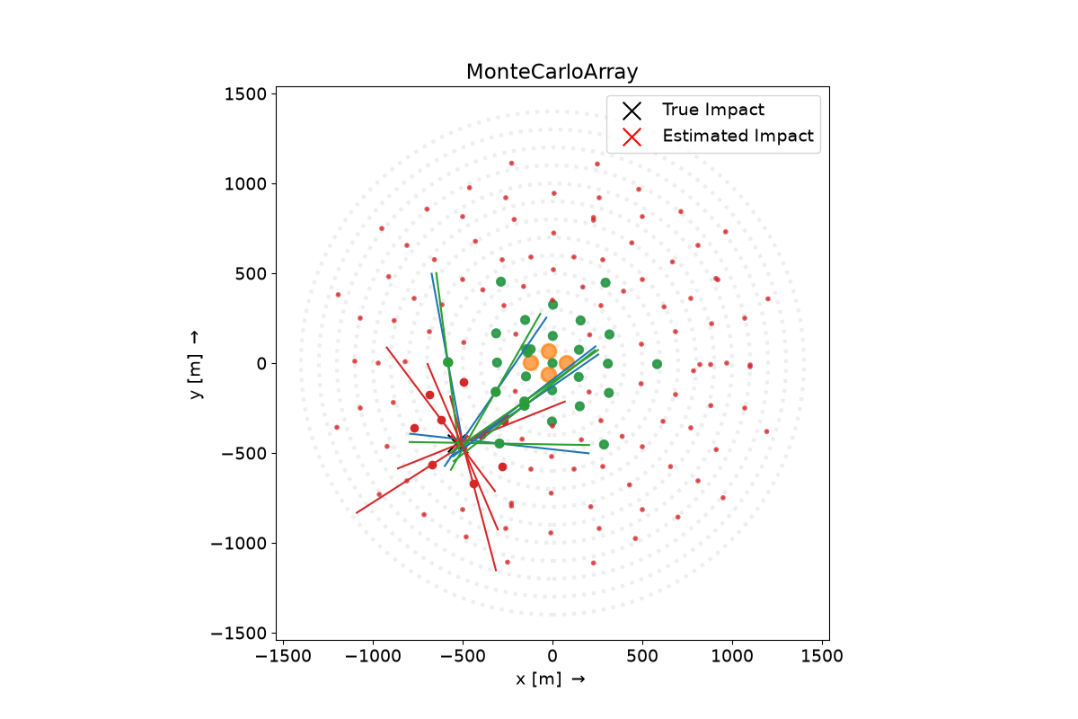
ArrayDisplay

angle_offset = plotting_event.monitoring.pointing.array_azimuth

plotting_hillas = {
    tel_id: dl1.parameters.hillas for tel_id, dl1 in plotting_event.dl1.tel.items()
}

plotting_core = {
    tel_id: dl1.parameters.core.psi for tel_id, dl1 in plotting_event.dl1.tel.items()
}


disp = ArrayDisplay(source.subarray)

disp.set_line_hillas(plotting_hillas, plotting_core, 500)

plt.scatter(
    plotting_event.simulation.shower.core_x,
    plotting_event.simulation.shower.core_y,
    s=200,
    c="k",
    marker="x",
    label="True Impact",
)
plt.scatter(
    plotting_event.dl2.stereo.geometry["HillasReconstructor"].core_x,
    plotting_event.dl2.stereo.geometry["HillasReconstructor"].core_y,
    s=200,
    c="r",
    marker="x",
    label="Estimated Impact",
)

plt.legend()
# plt.xlim(-400, 400)
# plt.ylim(-400, 400)

<matplotlib.legend.Legend object at 0x7c2221eb3020>

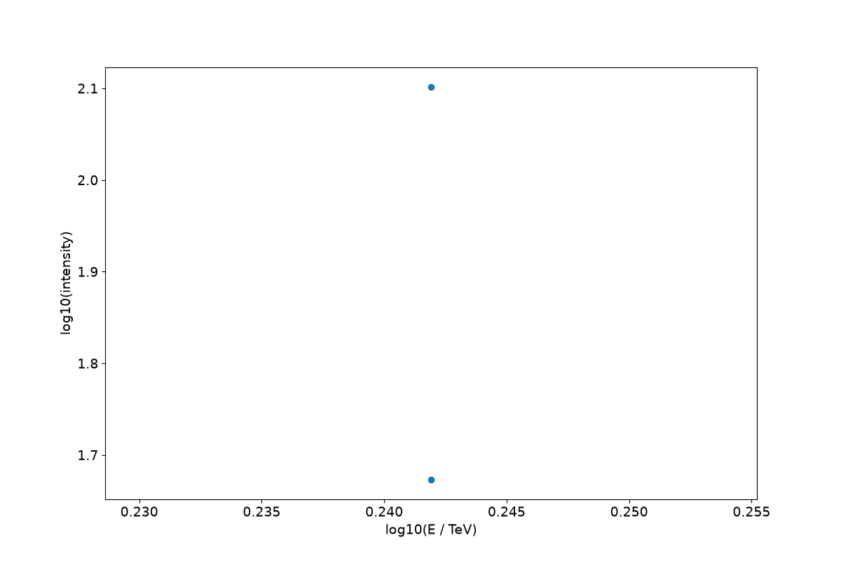
Reading the LST dl1 data

loader = TableLoader(f.name)

dl1_table = loader.read_telescope_events(
    ["LST_LST_LSTCam"],
    dl2=False,
    true_parameters=False,
)

plt.scatter(
    np.log10(dl1_table["true_energy"].quantity / u.TeV),
    np.log10(dl1_table["hillas_intensity"]),
)
plt.xlabel("log10(E / TeV)")
plt.ylabel("log10(intensity)")
None

Isn’t python slow?

• Many of you might have heard: “Python is slow”.

• That’s trueish.

• All python objects are classes living on the heap, even integers.

• Looping over lots of “primitives” is quite slow compared to other languages.

⇒ Vectorize as much as possible using numpy

⇒ Use existing interfaces to fast C / C++ / Fortran code

⇒ Optimize using numba

But: “Premature Optimization is the root of all evil” — Donald Knuth

So profile to find exactly what is slow.

Why use python then?

• Python works very well as glue for libraries of all kinds of languages

• Python has a rich ecosystem for data science, physics, algorithms, astronomy

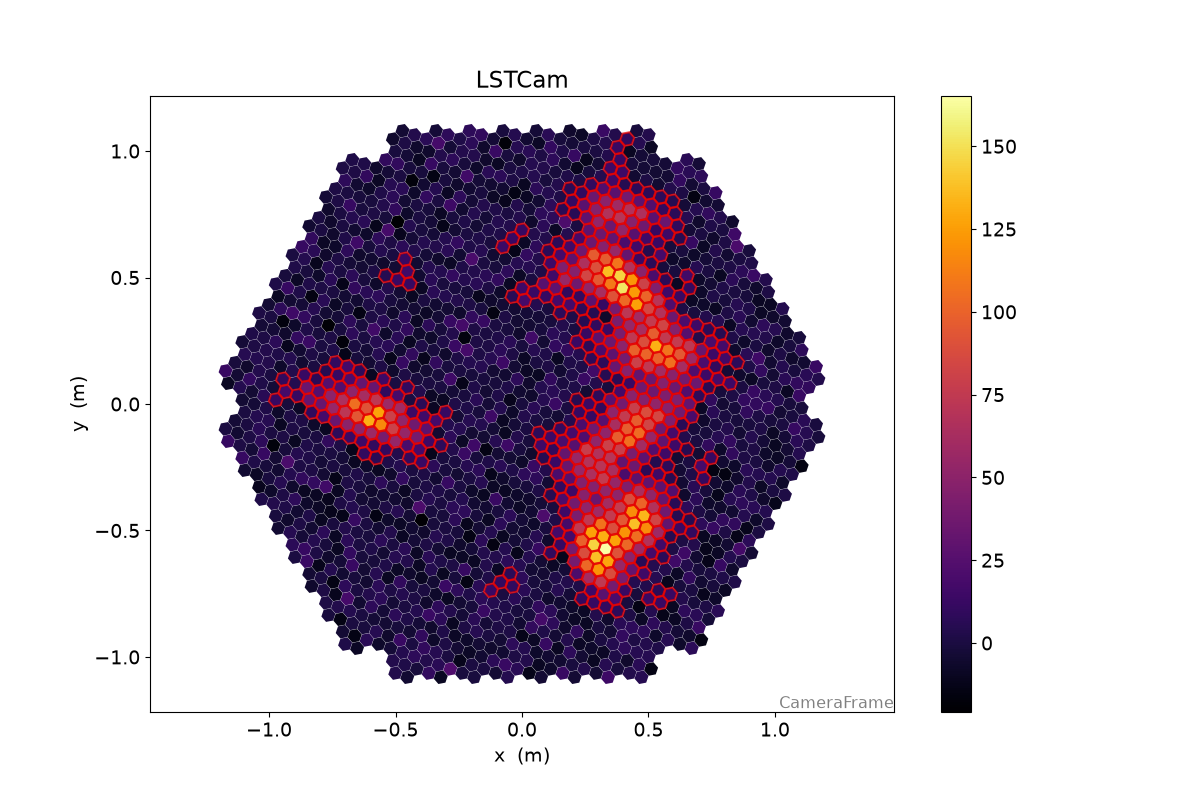
Example: Number of Islands

Find all groups of pixels, that survived the cleaning

geometry = loader.subarray.tel[1].camera.geometry

Let’s create a toy images with several islands;

rng = np.random.default_rng(42)

image = np.zeros(geometry.n_pixels)


for i in range(9):
    model = toymodel.Gaussian(
        x=rng.uniform(-0.8, 0.8) * u.m,
        y=rng.uniform(-0.8, 0.8) * u.m,
        width=rng.uniform(0.05, 0.075) * u.m,
        length=rng.uniform(0.1, 0.15) * u.m,
        psi=rng.uniform(0, 2 * np.pi) * u.rad,
    )

    new_image, sig, bg = model.generate_image(
        geometry, intensity=rng.uniform(1000, 3000), nsb_level_pe=5
    )
    image += new_image

clean = tailcuts_clean(
    geometry,
    image,
    picture_thresh=10,
    boundary_thresh=5,
    min_number_picture_neighbors=2,
)

disp = CameraDisplay(geometry)
disp.image = image
disp.highlight_pixels(clean, color="xkcd:red", linewidth=1.5)
disp.add_colorbar()

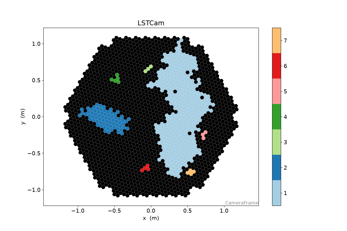
def num_islands_python(camera, clean):
    """A breadth first search to find connected islands of neighboring pixels in the cleaning set"""

    # the camera geometry has a [n_pixel, n_pixel] boolean array
    # that is True where two pixels are neighbors
    neighbors = camera.neighbor_matrix

    island_ids = np.zeros(camera.n_pixels)
    current_island = 0

    # a set to remember which pixels we already visited
    visited = set()

    # go only through the pixels, that survived cleaning
    for pix_id in np.where(clean)[0]:
        if pix_id not in visited:
            # remember that we already checked this pixel
            visited.add(pix_id)

            # if we land in the outer loop again, we found a new island
            current_island += 1
            island_ids[pix_id] = current_island

            # now check all neighbors of the current pixel recursively
            to_check = set(np.where(neighbors[pix_id] & clean)[0])
            while to_check:
                pix_id = to_check.pop()

                if pix_id not in visited:
                    visited.add(pix_id)
                    island_ids[pix_id] = current_island

                    to_check.update(np.where(neighbors[pix_id] & clean)[0])

    n_islands = current_island
    return n_islands, island_ids

n_islands, island_ids = num_islands_python(geometry, clean)

cmap = plt.get_cmap("Paired")
cmap = ListedColormap(cmap.colors[:n_islands])
cmap.set_under("k")

disp = CameraDisplay(geometry)
disp.image = island_ids
disp.cmap = cmap
disp.set_limits_minmax(0.5, n_islands + 0.5)
disp.add_colorbar()

timeit.timeit(lambda: num_islands_python(geometry, clean), number=1000) / 1000

0.001906123042001127

def num_islands_scipy(geometry, clean):
    neighbors = geometry.neighbor_matrix_sparse

    clean_neighbors = neighbors[clean][:, clean]
    num_islands, labels = connected_components(clean_neighbors, directed=False)

    island_ids = np.zeros(geometry.n_pixels)
    island_ids[clean] = labels + 1

    return num_islands, island_ids

n_islands_s, island_ids_s = num_islands_scipy(geometry, clean)

disp = CameraDisplay(geometry)
disp.image = island_ids_s
disp.cmap = cmap
disp.set_limits_minmax(0.5, n_islands_s + 0.5)
disp.add_colorbar()

timeit.timeit(lambda: num_islands_scipy(geometry, clean), number=10000) / 10000

0.0003123096999999689

A lot less code, and a factor 3 speed improvement

Finally, current ctapipe implementation is using numba:

timeit.timeit(lambda: number_of_islands(geometry, clean), number=100000) / 100000

1.6972994480001945e-05