Note
Go to the end to download the full example code.
Histogram aggregation with HistogramAggregator#
This tutorial shows how to:
Build an event table with camera-like data (images and peak times) and some invalid values.
Configure and run HistogramAggregator in chunks.
Access histogram counts, bin edges, summary statistics, and valid-event counts (n_events).
Plot one pixel histogram from the selected chunks and both gain channels for both image and peak_time columns.
Plot the same histogram using Hist’s built-in plotting functionality after filling a Hist object with the aggregated histogram counts and variances.
Plot the integral over all pixels for both channels using Hist’s built-in plotting functionality.
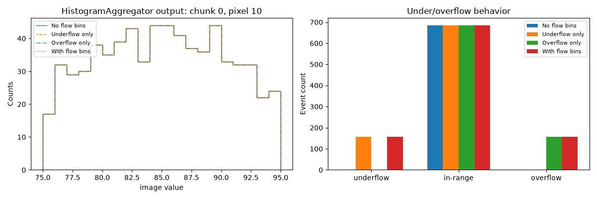
Compare no-flow, underflow-only, overflow-only, and both-flow histograms to see how the outer bins behave.
Number of chunks: 2
histogram shape per chunk: (50, 2, 100)
bin edges shape per chunk: (51,)
bin centers shape per chunk: (50,)
n_events shape per chunk: (2, 100)
16 import matplotlib.pyplot as plt
17 import numpy as np
18 from astropy.table import Table
19 from astropy.time import Time
20 from traitlets.config import Config
21
22 from ctapipe.containers import ChunkHistogramContainer
23 from ctapipe.monitoring.aggregator import HistogramAggregator
24
25
26 # -------------------------------------------------------------------
27 # Create synthetic event-wise camera data
28 # -------------------------------------------------------------------
29 rng = np.random.default_rng(42)
30
31 n_events = 2000
32 n_channels = 2
33 n_pixels = 100
34
35 times = Time(
36 np.linspace(60117.911, 60117.9258, num=n_events),
37 scale="tai",
38 format="mjd",
39 )
40 event_ids = np.arange(n_events)
41 images = rng.normal(loc=85.0, scale=10.0, size=(n_events, n_channels, n_pixels))
42 images[:, 1, :] -= 15 # Simulate lower gain channel by shifting the mean down by 15
43 peak_time = rng.normal(loc=20.0, scale=2.0, size=(n_events, n_channels, n_pixels))
44
45 # Add a few invalid values to demonstrate n_events behavior.
46 images[3, 0, 10] = np.nan
47 images[15, 0, 10] = np.nan
48 peak_time[5, 0, 10] = np.nan
49 peak_time[35, 1, 10] = np.nan
50
51 # Optional static mask over sample dimensions (channel, pixel).
52 # Here we exclude channel 1, pixel 99 for all events.
53 masked_elements_of_sample = np.zeros((n_channels, n_pixels), dtype=bool)
54 masked_elements_of_sample[1, 99] = True
55
56 table = Table(
57 [times, event_ids, images, peak_time],
58 names=("time", "event_id", "image", "peak_time"),
59 )
60
61
62 # -------------------------------------------------------------------
63 # Configure and run histogram aggregation
64 # -------------------------------------------------------------------
65 config_image = Config(
66 {
67 "HistogramAggregator": {
68 "chunking_type": "SizeChunking",
69 "axis_definition": {
70 "class_name": "Regular",
71 "bins": 50,
72 "start": 40.0,
73 "stop": 110.0,
74 "name": "image",
75 },
76 "axis_names": ["channel", "pixel"],
77 },
78 "SizeChunking": {"chunk_size": 1000},
79 }
80 )
81
82 aggregator_image = HistogramAggregator(config=config_image)
83 result = aggregator_image(
84 table=table,
85 col_name="image",
86 masked_elements_of_sample=masked_elements_of_sample,
87 )
88
89 config_peak_time = Config(
90 {
91 "HistogramAggregator": {
92 "chunking_type": "SizeChunking",
93 "axis_definition": {
94 "class_name": "Regular",
95 "bins": 50,
96 "start": 2.0,
97 "stop": 38.0,
98 "name": "peak_time",
99 },
100 "axis_names": ["channel", "pixel"],
101 },
102 "SizeChunking": {"chunk_size": 1000},
103 }
104 )
105
106 aggregator_peak_time = HistogramAggregator(config=config_peak_time)
107 result_peak_time = aggregator_peak_time(
108 table=table,
109 col_name="peak_time",
110 masked_elements_of_sample=masked_elements_of_sample,
111 )
112
113 print(f"Number of chunks: {len(result)}")
114 print(f"histogram shape per chunk: {result[0]['histogram'].shape}")
115 print(f"bin edges shape per chunk: {result[0].meta['bin_edges'].shape}")
116 print(f"bin centers shape per chunk: {result[0].meta['bin_centers'].shape}")
117 print(f"n_events shape per chunk: {result[0]['n_events'].shape}")
118
119
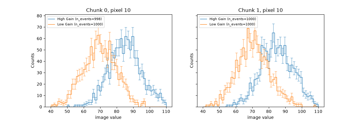
120 # -------------------------------------------------------------------
121 # Plot the histograms for one pixel with two gain channels
122 # -------------------------------------------------------------------
123 # We aggreagted the histograms in two chunks of 1000 events each, so we have two histograms per gain channel
124 # for the selected pixel. We will plot both chunks for the selected pixel and gain channels
125 # on the same axes for comparison, and then do the same for the peak_time column in a separate figure.
126
127 pixel_index = 10
128 gain_label = {0: "High Gain", 1: "Low Gain"}
129
130 fig, axes = plt.subplots(1, 2, figsize=(12, 4), sharey=True)
131 for chunk_index, ax in enumerate(axes):
132 bin_edges = result[chunk_index].meta["bin_edges"]
133 bin_centers = result[chunk_index].meta["bin_centers"]
134 channel_handles = []
135
136 for channel_index in range(n_channels):
137 counts = result[chunk_index]["histogram"][:, channel_index, pixel_index]
138 valid_events = result[chunk_index]["n_events"][channel_index, pixel_index]
139
140 line = ax.stairs(
141 counts,
142 bin_edges,
143 label=f"{gain_label[channel_index]} (n_events={valid_events})",
144 )
145 channel_handles.append(line)
146 color = line.get_edgecolor()
147
148 # Plot bin variances as error bars (use sqrt of variance for error) at bin centers
149 bin_errors = np.sqrt(counts)
150 ax.errorbar(
151 bin_centers,
152 counts,
153 yerr=bin_errors,
154 fmt="none",
155 color=color,
156 elinewidth=1.0,
157 capsize=3,
158 alpha=0.6,
159 )
160
161 ax.set_title(f"Chunk {chunk_index}, pixel {pixel_index}")
162 ax.set_xlabel("image value")
163 ax.set_ylabel("Counts")
164
165 ax.legend(
166 handles=channel_handles,
167 loc="upper left",
168 fontsize=8,
169 )
170
171 plt.show()
172
173
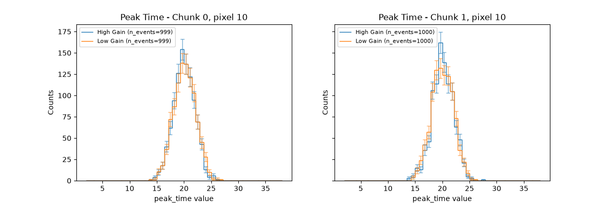
174 # -------------------------------------------------------------------
175 # Plot peak_time histograms in a separate figure
176 # -------------------------------------------------------------------
177 fig, axes = plt.subplots(1, 2, figsize=(12, 4), sharey=True)
178 for chunk_index, ax in enumerate(axes):
179 bin_edges = result_peak_time[chunk_index].meta["bin_edges"]
180 bin_centers = result_peak_time[chunk_index].meta["bin_centers"]
181
182 channel_handles = []
183
184 for channel_index in range(n_channels):
185 counts = result_peak_time[chunk_index]["histogram"][
186 :, channel_index, pixel_index
187 ]
188 valid_events = result_peak_time[chunk_index]["n_events"][
189 channel_index, pixel_index
190 ]
191
192 line = ax.stairs(
193 counts,
194 bin_edges,
195 label=f"{gain_label[channel_index]} (n_events={valid_events})",
196 )
197 channel_handles.append(line)
198 color = line.get_edgecolor()
199
200 # Plot bin variances as error bars (use sqrt of variance for error) at bin centers
201 bin_errors = np.sqrt(counts)
202 ax.errorbar(
203 bin_centers,
204 counts,
205 yerr=bin_errors,
206 fmt="none",
207 color=color,
208 elinewidth=1.0,
209 capsize=3,
210 alpha=0.6,
211 )
212
213 ax.set_title(f"Peak Time - Chunk {chunk_index}, pixel {pixel_index}")
214 ax.set_xlabel("peak_time value")
215 ax.set_ylabel("Counts")
216 ax.legend(
217 handles=channel_handles,
218 loc="upper left",
219 fontsize=8,
220 )
221
222 plt.show()
223
224
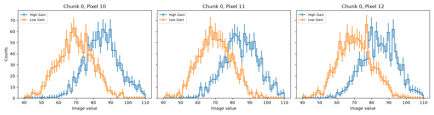
225 # -------------------------------------------------------------------
226 # Build a Hist object from serialized axis metadata and plot it
227 # -------------------------------------------------------------------
228
229 # Reconstruct the histogram axis from metadata stored by HistogramAggregator.
230 # In this tutorial, axis_definition uses hist.axis.Regular.
231 chunk_index = 0
232 chunk_histograms_container = ChunkHistogramContainer(
233 **dict(zip(result[chunk_index].colnames, result[chunk_index]))
234 )
235 chunk_histograms_container.meta = result.meta
236
237 # Plot three nearby pixels using Hist's built-in plotting functionality.
238 # Requires 'hist[plot]' to be installed in the environment. Reconstruct
239 # the full histogram as a Hist object for the chunk using hist_from_container method.
240 full_hist = HistogramAggregator.hist_from_container(chunk_histograms_container)
241 pixels_to_plot = [pixel_index, pixel_index + 1, pixel_index + 2]
242 fig, axes = plt.subplots(1, len(pixels_to_plot), figsize=(15, 4), sharey=True)
243
244 for ax, pixel_to_plot in zip(axes, pixels_to_plot):
245 for channel_index in range(n_channels):
246 h = full_hist[{"channel": channel_index, "pixel": pixel_to_plot}]
247 h.name = gain_label[channel_index]
248
249 plt.sca(ax)
250 h.plot(histtype="step", yerr=True, label=h.name)
251
252 ax.set_title(f"Chunk {chunk_index}, Pixel {pixel_to_plot}")
253 ax.set_xlabel("image value")
254 ax.legend(fontsize=8, loc="upper left")
255
256 axes[0].set_ylabel("Counts")
257 plt.tight_layout()
258 plt.show()
259
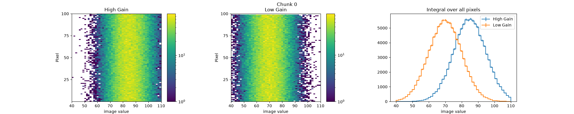
260 # ------------------------------------------------------------------------------------------------
261 # Plot the integral over all pixels for both channels using Hist's built-in plotting functionality
262 # ------------------------------------------------------------------------------------------------
263 h = full_hist
264
265 fig, ax = plt.subplots(
266 1,
267 3,
268 figsize=(20, 4),
269 gridspec_kw={"width_ratios": [1.15, 1.15, 1.4]},
270 )
271 fig.suptitle(f"Chunk {chunk_index}")
272 h[:, 0, :].plot2d(ax=ax[0], norm="log")
273 h[:, 1, :].plot2d(ax=ax[1], norm="log")
274 channel_stack = h.integrate("pixel").stack("channel")
275 channel_stack[0].name = "High Gain"
276 channel_stack[1].name = "Low Gain"
277 channel_stack.plot(ax=ax[2], legend=True)
278
279 ax[0].set_title(channel_stack[0].name)
280 ax[1].set_title(channel_stack[1].name)
281 ax[2].set_title("Integral over all pixels")
282 for heatmap_ax in ax[:2]:
283 heatmap_ax.set_xlabel("image value")
284 heatmap_ax.set_ylabel("Pixel")
285 heatmap_ax.set_yticks([25, 50, 75, 100], labels=["25", "50", "75", "100"])
286
287 ax[2].set_xlabel("image value")
288 fig.subplots_adjust(wspace=0.5, top=0.88)
289 plt.show()
290
291 # ----------------------------------------------------------------------
292 # Demonstrate underflow/overflow via HistogramAggregator axis_definition
293 # ----------------------------------------------------------------------
294
295 FLOW_CONFIGS = {
296 "No flow bins": {"underflow": False, "overflow": False},
297 "Underflow only": {"underflow": True, "overflow": False},
298 "Overflow only": {"underflow": False, "overflow": True},
299 "With flow bins": {"underflow": True, "overflow": True},
300 }
301
302 BASE_AXIS = {
303 "class_name": "Regular",
304 "bins": 20,
305 "start": 75.0,
306 "stop": 95.0,
307 }
308
309 CHUNKING = {
310 "chunking_type": "SizeChunking",
311 "SizeChunking": {"chunk_size": 1000},
312 }
313 # Run all configurations and extract histograms/counts
314 results = {}
315 histograms = {}
316 flow_counts = {}
317
318 for label, flow_options in FLOW_CONFIGS.items():
319 config = Config(
320 {
321 "HistogramAggregator": {
322 "chunking_type": "SizeChunking",
323 "axis_definition": {
324 **BASE_AXIS,
325 **flow_options,
326 },
327 "axis_names": ["channel", "pixel"],
328 },
329 "SizeChunking": {"chunk_size": 1000},
330 }
331 )
332
333 # Aggregate the histogram which will return an astropy table
334 result = HistogramAggregator(config=config)(
335 table=table,
336 col_name="image",
337 masked_elements_of_sample=masked_elements_of_sample,
338 )
339 # Create a Hist object from the aggregated histogram and
340 # metadata for the selected chunk using the hist_from_tablerow method.
341 histogram_cont = HistogramAggregator.hist_from_tablerow(result[chunk_index])
342 histogram = histogram_cont[{"channel": 0, "pixel": pixel_index}]
343
344 flow_view = histogram.view(flow=True)
345 axis_kwargs = result.meta["axis_kwargs"]
346
347 results[label] = result
348 histograms[label] = histogram
349 flow_counts[label] = {
350 "underflow": (int(flow_view[0]) if axis_kwargs.get("underflow") else 0),
351 "in_range": int(histogram.values().sum()),
352 "overflow": (int(flow_view[-1]) if axis_kwargs.get("overflow") else 0),
353 }
354
355 valid_events = results["With flow bins"][chunk_index]["n_events"][0, pixel_index]
356
357 fig, axes = plt.subplots(1, 2, figsize=(12, 4))
358
359 styles = {
360 "No flow bins": "-",
361 "Underflow only": "--",
362 "Overflow only": "-.",
363 "With flow bins": ":",
364 }
365
366 # Left: histogram comparison
367 for label, histogram in histograms.items():
368 axes[0].stairs(
369 histogram.values(),
370 histogram.axes[0].edges,
371 linestyle=styles[label],
372 label=label,
373 )
374
375 axes[0].set_title(
376 f"HistogramAggregator output: chunk {chunk_index}, pixel {pixel_index}"
377 )
378 axes[0].set_xlabel("image value")
379 axes[0].set_ylabel("Counts")
380
381 axis_margin = 0.05 * (BASE_AXIS["stop"] - BASE_AXIS["start"])
382 axes[0].set_xlim(
383 BASE_AXIS["start"] - axis_margin,
384 BASE_AXIS["stop"] + axis_margin,
385 )
386
387 axes[0].legend(fontsize=8, loc="upper left")
388
389 # Right: flow-bin behavior
390 x = np.arange(3)
391 labels = ["underflow", "in-range", "overflow"]
392
393 bar_offsets = {
394 "No flow bins": -0.18,
395 "Underflow only": 0.00,
396 "Overflow only": 0.18,
397 "With flow bins": 0.36,
398 }
399
400 bar_width = 0.18
401
402 for label, offset in bar_offsets.items():
403 counts = flow_counts[label]
404
405 axes[1].bar(
406 x + offset,
407 [
408 counts["underflow"],
409 counts["in_range"],
410 counts["overflow"],
411 ],
412 width=bar_width,
413 label=label,
414 )
415
416 axes[1].set_xticks(x + 0.09, labels)
417 axes[1].set_ylabel("Event count")
418 axes[1].set_title("Under/overflow behavior")
419 axes[1].legend(fontsize=8)
420
421 plt.tight_layout()
422 plt.show()
Total running time of the script: (0 minutes 2.038 seconds)