Exploring Raw Data

Here are just some very simple examples of going through and inspecting the raw data, and making some plots using ctapipe. The data explored here are raw Monte Carlo data, which is Data Level “R0” in CTA terminology (e.g. it is before any processing that would happen inside a Camera or off-line)

Setup:

from ctapipe.utils import get_dataset_path
from ctapipe.io import EventSource
from ctapipe.visualization import CameraDisplay
from ctapipe.instrument import CameraGeometry
from matplotlib import pyplot as plt
from astropy import units as u

%matplotlib inline

To read SimTelArray format data, ctapipe uses the pyeventio library (which is installed automatically along with ctapipe). The following lines however will load any data known to ctapipe (multiple EventSources are implemented, and chosen automatically based on the type of the input file.

All data access first starts with an EventSource, and here we use a helper function event_source that constructs one. The resulting source object can be iterated over like a list of events. We also here use an EventSeeker which provides random-access to the source (by seeking to the given event ID or number)

source = EventSource(get_dataset_path("gamma_prod5.simtel.zst"), max_events=5)

Explore the contents of an event

note that the R0 level is the raw data that comes out of a camera, and also the lowest level of monte-carlo data.

# so we can advance through events one-by-one
event_iterator = iter(source)

event = next(event_iterator)

the event is just a class with a bunch of data items in it. You can see a more compact represntation via:

event.r0

ctapipe.containers.R0Container:
                        tel[*]: map of tel_id to R0CameraContainer with default
                                None

printing the event structure, will currently print the value all items under it (so you get a lot of output if you print a high-level container):

print(event.simulation.shower)

{'alt': <Angle 1.22173047 rad>,
 'az': <Angle 6.28318501 rad>,
 'core_x': <Quantity -146.42298889 m>,
 'core_y': <Quantity 341.64358521 m>,
 'energy': <Quantity 0.07287972 TeV>,
 'h_first_int': <Quantity 32396.98828125 m>,
 'shower_primary_id': 0,
 'x_max': <Quantity 159.41175842 g / cm2>}

print(event.r0.tel.keys())

dict_keys([9, 14, 104])

note that the event has 3 telescopes in it: Let’s try the next one:

event = next(event_iterator)
print(event.r0.tel.keys())

dict_keys([26, 27, 29, 47, 53, 59, 69, 73, 121, 122, 124, 148, 162, 166])

now, we have a larger event with many telescopes… Let’s look at one of them:

teldata = event.r0.tel[26]
print(teldata)
teldata

{'waveform': array([[[267, 276, 282, ..., 237, 246, 259],
        [254, 249, 254, ..., 210, 208, 208],
        [214, 233, 254, ..., 271, 272, 272],
        ...,
        [242, 236, 228, ..., 242, 252, 259],
        [245, 236, 230, ..., 248, 246, 248],
        [229, 231, 233, ..., 236, 238, 234]]], dtype=uint16)}

ctapipe.containers.R0CameraContainer:
                      waveform: numpy array containing ADC samples(n_channels,
                                n_pixels, n_samples) with default None

Note that some values are unit quantities (astropy.units.Quantity) or angular quantities (astropy.coordinates.Angle), and you can easily maniuplate them:

event.simulation.shower.energy

$1.7454714 \; \mathrm{TeV}$

event.simulation.shower.energy.to('GeV')

$1745.4714 \; \mathrm{GeV}$

event.simulation.shower.energy.to('J')

$2.7965534 \times 10^{-7} \; \mathrm{J}$

event.simulation.shower.alt

$1.22173\mathrm{rad}$

print("Altitude in degrees:", event.simulation.shower.alt.deg)

Altitude in degrees: 69.99999967119774

Look for signal pixels in a camera

again, event.r0.tel[x] contains a data structure for the telescope data, with some fields like waveform.

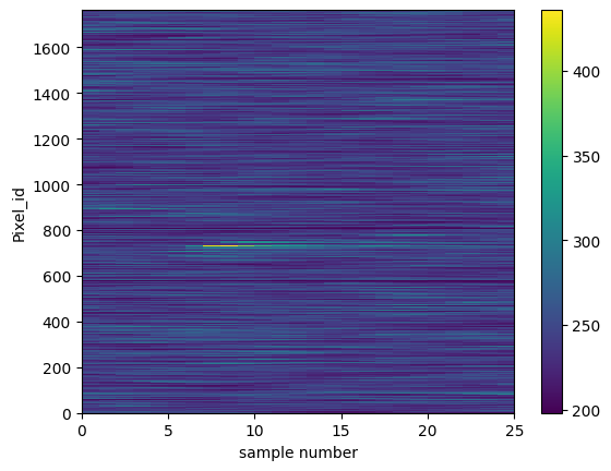
Let’s make a 2D plot of the sample data (sample vs pixel), so we can see if we see which pixels contain Cherenkov light signals:

plt.pcolormesh(teldata.waveform[0])  # note the [0] is for channel 0
plt.colorbar()
plt.xlabel("sample number")
plt.ylabel("Pixel_id")

Text(0, 0.5, 'Pixel_id')

Let’s zoom in to see if we can identify the pixels that have the Cherenkov signal in them

plt.pcolormesh(teldata.waveform[0])
plt.colorbar()
plt.ylim(700,750)
plt.xlabel("sample number")
plt.ylabel("pixel_id")
print("waveform[0] is an array of shape (N_pix,N_slice) =",teldata.waveform[0].shape)

waveform[0] is an array of shape (N_pix,N_slice) = (1764, 25)

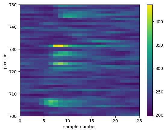
Now we can really see that some pixels have a signal in them!

Lets look at a 1D plot of pixel 270 in channel 0 and see the signal:

trace = teldata.waveform[0][719]
plt.plot(trace, drawstyle='steps')

[<matplotlib.lines.Line2D at 0x7f351444d5e0>]

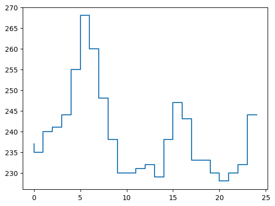
Great! It looks like a standard Cherenkov signal!

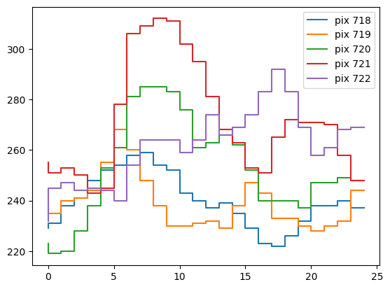
Let’s take a look at several traces to see if the peaks area aligned:

for pix_id in range(718,723):
    plt.plot(teldata.waveform[0][pix_id], label="pix {}".format(pix_id), drawstyle='steps')
plt.legend()

<matplotlib.legend.Legend at 0x7f3514d55400>

Look at the time trace from a Camera Pixel

ctapipe.calib.camera includes classes for doing automatic trace integration with many methods, but before using that, let’s just try to do something simple!

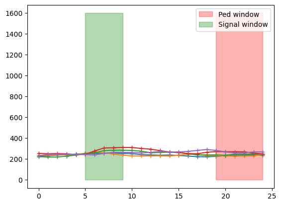
Let’s define the integration windows first: By eye, they seem to be reaonsable from sample 8 to 13 for signal, and 20 to 29 for pedestal (which we define as the sum of all noise: NSB + electronic)

for pix_id in range(718,723):
    plt.plot(teldata.waveform[0][pix_id],'+-')
plt.fill_betweenx([0,1600],19,24,color='red',alpha=0.3, label='Ped window')
plt.fill_betweenx([0,1600],5,9,color='green',alpha=0.3, label='Signal window')
plt.legend()

<matplotlib.legend.Legend at 0x7f351434d280>

Do a very simplisitic trace analysis

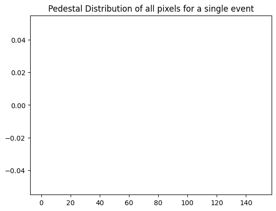
Now, let’s for example calculate a signal and background in a the fixed windows we defined for this single event. Note we are ignoring the fact that cameras have 2 gains, and just using a single gain (channel 0, which is the high-gain channel):

data = teldata.waveform[0]
peds = data[:, 19:24].mean(axis=1)  # mean of samples 20 to 29 for all pixels
sums = data[:, 5:9].sum(axis=1)/(13-8)    # simple sum integration

phist = plt.hist(peds, bins=50, range=[0,150])
plt.title("Pedestal Distribution of all pixels for a single event")

Text(0.5, 1.0, 'Pedestal Distribution of all pixels for a single event')

let’s now take a look at the pedestal-subtracted sums and a pedestal-subtracted signal:

plt.plot(sums - peds)
plt.xlabel("pixel id")
plt.ylabel("Pedestal-subtracted Signal")

Text(0, 0.5, 'Pedestal-subtracted Signal')

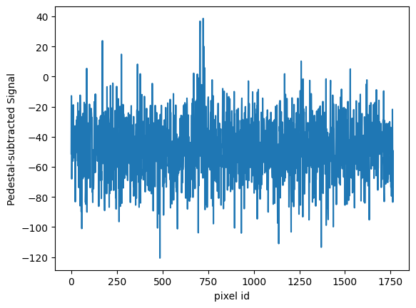
Now, we can clearly see that the signal is centered at 0 where there is no Cherenkov light, and we can also clearly see the shower around pixel 250.

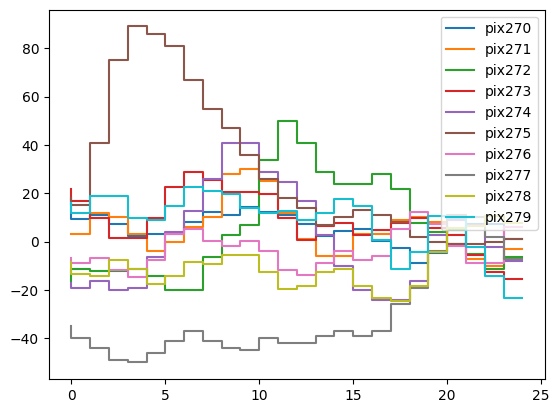
# we can also subtract the pedestals from the traces themselves, which would be needed to compare peaks properly
for ii in range(270,280):
    plt.plot(data[ii] - peds[ii], drawstyle='steps', label="pix{}".format(ii))
plt.legend()

<matplotlib.legend.Legend at 0x7f351423c190>

Camera Displays

It’s of course much easier to see the signal if we plot it in 2D with correct pixel positions!

note: the instrument data model is not fully implemented, so there is not a good way to load all the camera information (right now it is hacked into the inst sub-container that is read from the Monte-Carlo file)

camgeom = source.subarray.tel[24].camera.geometry

title="CT24, run {} event {} ped-sub".format(event.index.obs_id,event.index.event_id)
disp = CameraDisplay(camgeom,title=title)
disp.image = sums - peds
disp.cmap = plt.cm.RdBu_r
disp.add_colorbar()
disp.set_limits_percent(95)  # autoscale

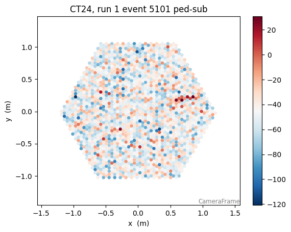
It looks like a nice signal! We have plotted our pedestal-subtracted trace integral, and see the shower clearly!

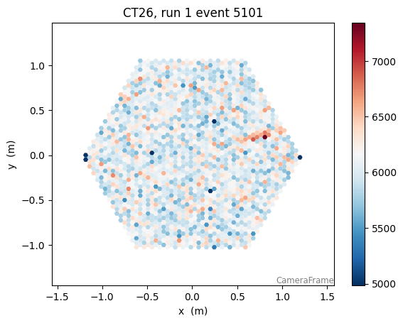
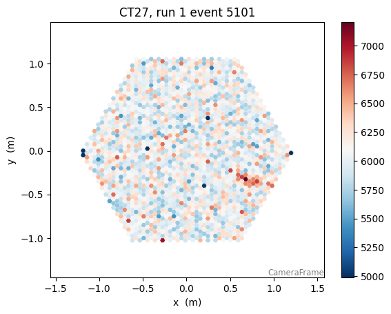
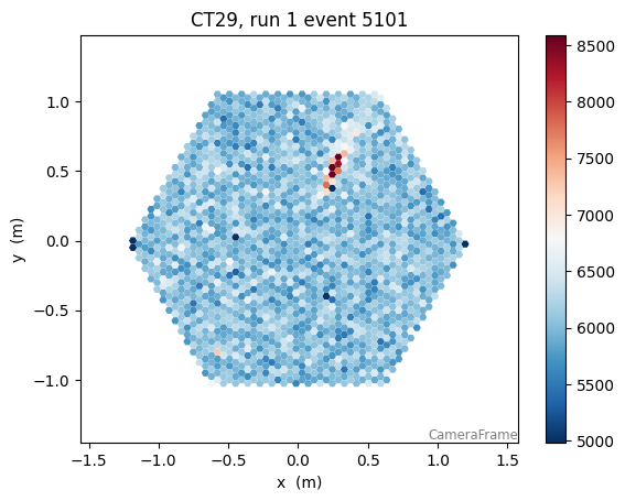
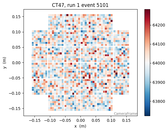
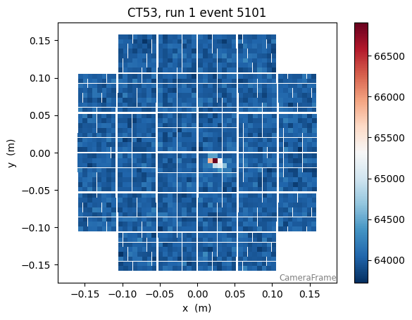
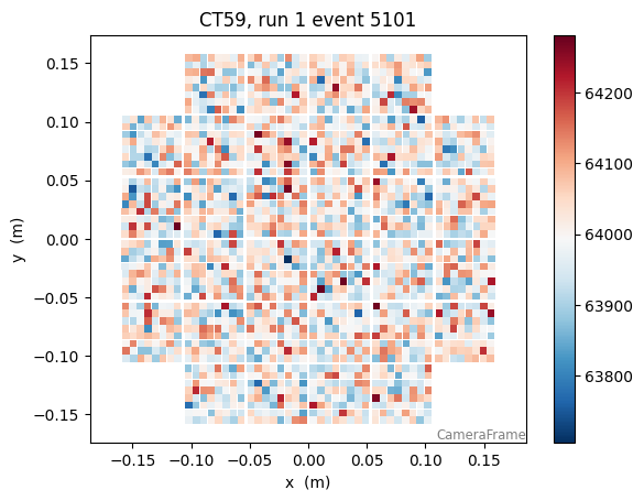
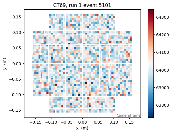
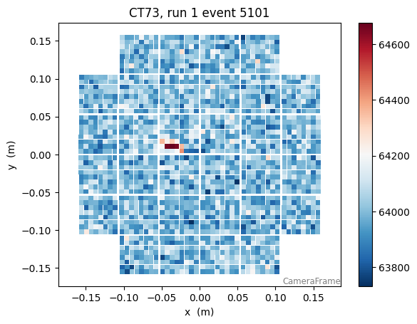
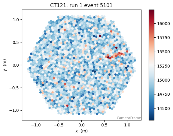
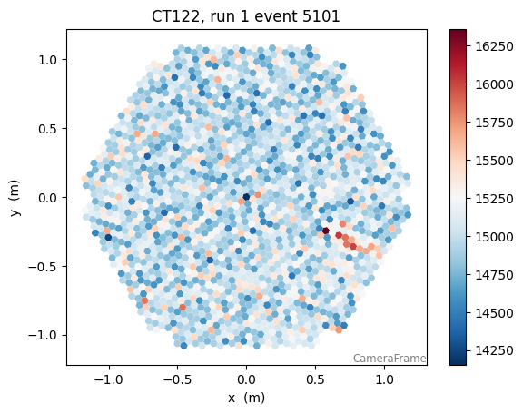
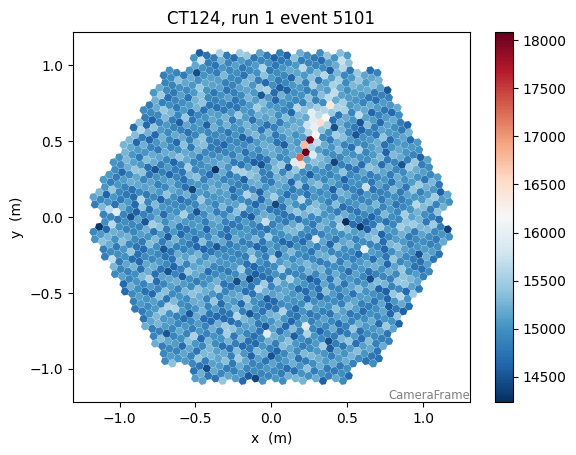
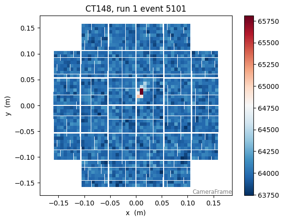
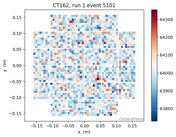
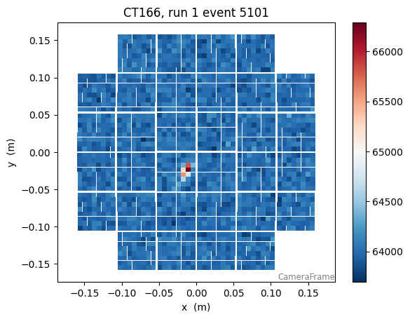
Let’s look at all telescopes:

note we plot here the raw signal, since we have not calculated the pedestals for each)

for tel in event.r0.tel.keys():
    plt.figure()
    camgeom = source.subarray.tel[tel].camera.geometry
    title="CT{}, run {} event {}".format(tel,event.index.obs_id,event.index.event_id)
    disp = CameraDisplay(camgeom,title=title)
    disp.image = event.r0.tel[tel].waveform[0].sum(axis=1)
    disp.cmap = plt.cm.RdBu_r
    disp.add_colorbar()
    disp.set_limits_percent(95)

some signal processing…

Let’s try to detect the peak using the scipy.signal package: https://docs.scipy.org/doc/scipy/reference/signal.html

from scipy import signal
import numpy as np

pix_ids = np.arange(len(data))
has_signal = sums > 300

widths = np.array([8,]) # peak widths to search for (let's fix it at 8 samples, about the width of the peak)
peaks = [signal.find_peaks_cwt(trace,widths) for trace in data[has_signal] ]

for p,s in zip(pix_ids[has_signal],peaks):
    print("pix{} has peaks at sample {}".format(p,s))
    plt.plot(data[p], drawstyle='steps-mid')
    plt.scatter(np.array(s),data[p,s])

clearly the signal needs to be filtered first, or an appropriate wavelet used, but the idea is nice