Analyzing Events Using ctapipe
![]()
Initially presented @ LST Analysis Bootcamp
Padova, 26.11.2018
Maximilian Nöthe (@maxnoe) & Kai A. Brügge (@mackaiver)
[1]:
import matplotlib.pyplot as plt
import numpy as np

%matplotlib inline
[2]:
plt.rcParams["figure.figsize"] = (12, 8)
plt.rcParams["font.size"] = 14
plt.rcParams["figure.figsize"]
[2]:
[12.0, 8.0]
Table of Contents
General Information
Design
DL0 → DL3 analysis
Currently some R0 → DL2 code to be able to analyze simtel files
ctapipe is built upon the Scientific Python Stack, core dependencies are
numpy
scipy
astropy
numba
Developement
ctapipe is developed as Open Source Software (BSD 3-Clause License) at https://github.com/cta-observatory/ctapipe
We use the “Github-Workflow”:
Few people (e.g. @kosack, @maxnoe) have write access to the main repository
Contributors fork the main repository and work on branches
Pull Requests are merged after Code Review and automatic execution of the test suite
Early developement stage ⇒ backwards-incompatible API changes might and will happen
What’s there?
Reading simtel simulation files
Simple calibration, cleaning and feature extraction functions
Camera and Array plotting
Coordinate frames and transformations
Stereo-reconstruction using line intersections
What’s still missing?
Good integration with machine learning techniques
IRF calculation
Documentation, e.g. formal definitions of coordinate frames
What can you do?
Report issues
Hard to get started? Tell us where you are stuck
Tell user stories
Missing features
Start contributing
ctapipe needs more workpower
Implement new reconstruction features
A simple hillas analysis
Reading in simtel files
[3]:
from ctapipe.io import EventSource
from ctapipe.utils.datasets import get_dataset_path

input_url = get_dataset_path("gamma_prod5.simtel.zst")

# EventSource() automatically detects what kind of file we are giving it,
# if already supported by ctapipe
source = EventSource(input_url, max_events=5)

print(type(source))
<class 'ctapipe.io.simteleventsource.SimTelEventSource'>
[4]:
for event in source:
    print(
        "Id: {}, E = {:1.3f}, Telescopes: {}".format(
            event.count, event.simulation.shower.energy, len(event.r0.tel)
        )
    )
Id: 0, E = 0.073 TeV, Telescopes: 3
Id: 1, E = 1.745 TeV, Telescopes: 14
Id: 2, E = 1.745 TeV, Telescopes: 4
Id: 3, E = 1.745 TeV, Telescopes: 20
Id: 4, E = 1.745 TeV, Telescopes: 31
Each event is a DataContainer holding several Fields of data, which can be containers or just numbers. Let’s look a one event:
[5]:
event
[5]:
ctapipe.containers.ArrayEventContainer:
                       index.*: event indexing information with default None
                          r0.*: Raw Data with default None
                          r1.*: R1 Calibrated Data with default None
                         dl0.*: DL0 Data Volume Reduced Data with default None
                         dl1.*: DL1 Calibrated image with default None
                         dl2.*: DL2 reconstruction info with default None
                  simulation.*: Simulated Event Information with default None
                                with type <class
                                'ctapipe.containers.SimulatedEventContainer'>
                     trigger.*: central trigger information with default None
                         count: number of events processed with default 0
                    pointing.*: Array and telescope pointing positions with
                                default None
                 calibration.*: Container for calibration coefficients for the
                                current event with default None
                         mon.*: container for event-wise monitoring data (MON)
                                with default None
                        muon.*: Container for muon analysis results with default
                                None
[6]:
source.subarray.camera_types
[6]:
(CameraDescription(name=CHEC, geometry=CHEC, readout=CHEC),
 CameraDescription(name=FlashCam, geometry=FlashCam, readout=FlashCam),
 CameraDescription(name=LSTCam, geometry=LSTCam, readout=LSTCam),
 CameraDescription(name=NectarCam, geometry=NectarCam, readout=NectarCam))
[7]:
len(event.r0.tel), len(event.r1.tel)
[7]:
(31, 31)
Data calibration
The CameraCalibrator calibrates the event (obtaining the dl1 images).
[8]:
from ctapipe.calib import CameraCalibrator

calibrator = CameraCalibrator(subarray=source.subarray)
[9]:
calibrator(event)
Event displays
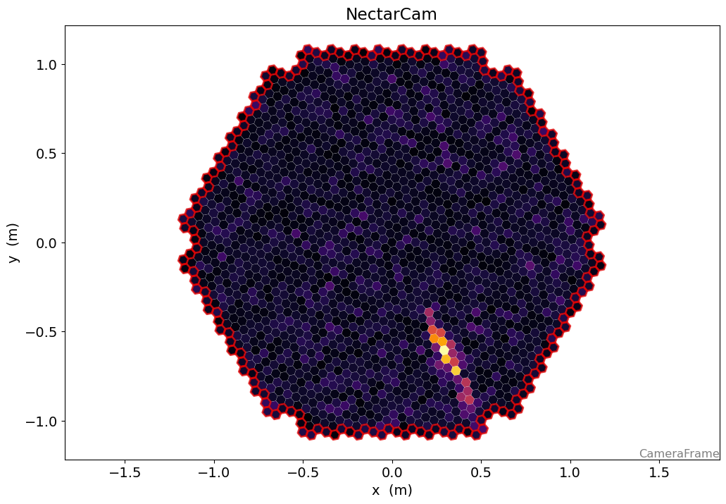
Let’s use ctapipe’s plotting facilities to plot the telescope images
[10]:
event.dl1.tel.keys()
[10]:
dict_keys([3, 4, 8, 9, 14, 15, 23, 24, 25, 29, 32, 36, 42, 46, 52, 56, 103, 104, 109, 110, 118, 119, 120, 126, 127, 129, 130, 137, 139, 143, 161])
[11]:
tel_id = 130
[12]:
geometry = source.subarray.tel[tel_id].camera.geometry
dl1 = event.dl1.tel[tel_id]

geometry, dl1
[12]:
(CameraGeometry(name='NectarCam', pix_type=PixelShape.HEXAGON, npix=1855, cam_rot=0.000 deg, pix_rot=40.893 deg, frame=<CameraFrame Frame (focal_length=16.445049285888672 m, rotation=0.0 rad, telescope_pointing=None, obstime=None, location=None)>),
 ctapipe.containers.DL1CameraContainer:
                          image: Numpy array of camera image, after waveform
                                 extraction.Shape: (n_pixel) with default None as
                                 a 1-D array with dtype float32
                      peak_time: Numpy array containing position of the peak of
                                 the pulse as determined by the extractor. Shape:
                                 (n_pixel, ) with default None as a 1-D array
                                 with dtype float32
                     image_mask: Boolean numpy array where True means the pixel
                                 has passed cleaning. Shape: (n_pixel, ) with
                                 default None as a 1-D array with dtype bool
                       is_valid: True if image extraction succeeded, False if
                                 failed or in the case of TwoPass methods, that
                                 the first pass only was returned. with default
                                 False
                     parameters: Image parameters with default None with type
                                 <class
                                 'ctapipe.containers.ImageParametersContainer'>)
[13]:
dl1.image
[13]:
array([-0.3856395 ,  1.2851689 ,  1.403967  , ...,  2.6847053 ,
        0.04941979, -1.0566036 ], dtype=float32)
[14]:
from ctapipe.visualization import CameraDisplay

display = CameraDisplay(geometry)

# right now, there might be one image per gain channel.
# This will change as soon as
display.image = dl1.image
display.add_colorbar()
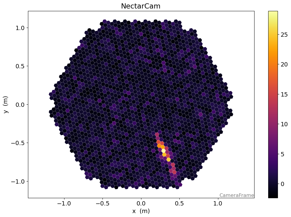
Image Cleaning
[15]:
from ctapipe.image.cleaning import tailcuts_clean
[16]:
# unoptimized cleaning levels
cleaning_level = {
    "CHEC": (2, 4, 2),
    "LSTCam": (3.5, 7, 2),
    "FlashCam": (3.5, 7, 2),
    "NectarCam": (4, 8, 2),
}
[17]:
boundary, picture, min_neighbors = cleaning_level[geometry.name]

clean = tailcuts_clean(
    geometry,
    dl1.image,
    boundary_thresh=boundary,
    picture_thresh=picture,
    min_number_picture_neighbors=min_neighbors,
)
[18]:
fig, (ax1, ax2) = plt.subplots(1, 2, figsize=(15, 5))

d1 = CameraDisplay(geometry, ax=ax1)
d2 = CameraDisplay(geometry, ax=ax2)

ax1.set_title("Image")
d1.image = dl1.image
d1.add_colorbar(ax=ax1)

ax2.set_title("Pulse Time")
d2.image = dl1.peak_time - np.average(dl1.peak_time, weights=dl1.image)
d2.cmap = "RdBu_r"
d2.add_colorbar(ax=ax2)
d2.set_limits_minmax(-20, 20)

d1.highlight_pixels(clean, color="red", linewidth=1)
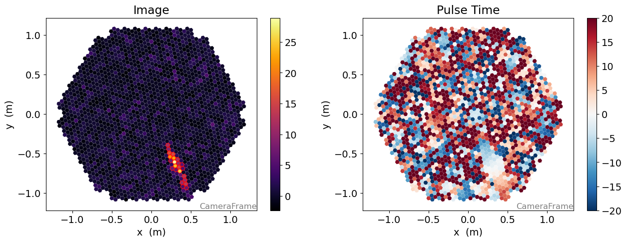
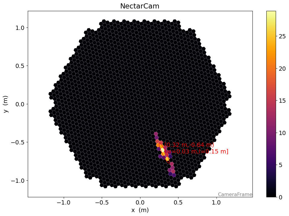
Image Parameters
[19]:
from ctapipe.image import (
    hillas_parameters,
    leakage_parameters,
    concentration_parameters,
)
from ctapipe.image import timing_parameters
from ctapipe.image import number_of_islands
from ctapipe.image import camera_to_shower_coordinates
[20]:
hillas = hillas_parameters(geometry[clean], dl1.image[clean])

print(hillas)
{'intensity': 303.9444303512573,
 'kurtosis': 2.464947780881624,
 'length': <Quantity 0.14667835 m>,
 'length_uncertainty': <Quantity 0.00509155 m>,
 'phi': <Angle -1.11344351 rad>,
 'psi': <Angle -1.12308339 rad>,
 'r': <Quantity 0.71788425 m>,
 'skewness': 0.3609063798795416,
 'width': <Quantity 0.02584731 m>,
 'width_uncertainty': <Quantity 0.00111159 m>,
 'x': <Quantity 0.31699941 m>,
 'y': <Quantity -0.64410339 m>}
[21]:
display = CameraDisplay(geometry)

# set "unclean" pixels to 0
cleaned = dl1.image.copy()
cleaned[~clean] = 0.0

display.image = cleaned
display.add_colorbar()

display.overlay_moments(hillas, color="xkcd:red")
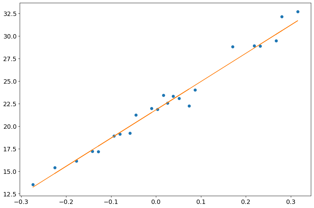
[22]:
timing = timing_parameters(geometry, dl1.image, dl1.peak_time, hillas, clean)

print(timing)
{'deviation': 0.7921518270503362,
 'intercept': 21.812572562414946,
 'slope': <Quantity 31.32320575 1 / m>}
[23]:
long, trans = camera_to_shower_coordinates(
    geometry.pix_x, geometry.pix_y, hillas.x, hillas.y, hillas.psi
)

plt.plot(long[clean], dl1.peak_time[clean], "o")
plt.plot(long[clean], timing.slope * long[clean] + timing.intercept)
[23]:
[<matplotlib.lines.Line2D at 0x7f4124dc3400>]
[24]:
l = leakage_parameters(geometry, dl1.image, clean)
print(l)
{'intensity_width_1': 0.0,
 'intensity_width_2': 0.0,
 'pixels_width_1': 0.0,
 'pixels_width_2': 0.0}
[25]:
disp = CameraDisplay(geometry)
disp.image = dl1.image
disp.highlight_pixels(geometry.get_border_pixel_mask(1), linewidth=2, color="xkcd:red")
[26]:
n_islands, island_id = number_of_islands(geometry, clean)

print(n_islands)
2
[27]:
conc = concentration_parameters(geometry, dl1.image, hillas)
print(conc)
{'cog': 0.2571728392782083,
 'core': 0.4014042974365615,
 'pixel': 0.09514053791448862}
Putting it all together / Stereo reconstruction
All these steps are now unified in several components configurable through the config system, mainly:
CameraCalibrator for DL0 → DL1 (Images)
ImageProcessor for DL1 (Images) → DL1 (Parameters)
ShowerProcessor for stereo reconstruction of the shower geometry
DataWriter for writing data into HDF5
A command line tool doing these steps and writing out data in HDF5 format is available as ctapipe-process
[28]:
import astropy.units as u
from astropy.coordinates import SkyCoord, AltAz

from ctapipe.containers import ImageParametersContainer
from ctapipe.io import EventSource
from ctapipe.utils.datasets import get_dataset_path

from ctapipe.calib import CameraCalibrator

from ctapipe.image import ImageProcessor
from ctapipe.reco import ShowerProcessor

from ctapipe.io import DataWriter

from copy import deepcopy
import tempfile

from traitlets.config import Config


image_processor_config = Config(
    {
        "ImageProcessor": {
            "image_cleaner_type": "TailcutsImageCleaner",
            "TailcutsImageCleaner": {
                "picture_threshold_pe": [
                    ("type", "LST_LST_LSTCam", 7.5),
                    ("type", "MST_MST_FlashCam", 8),
                    ("type", "MST_MST_NectarCam", 8),
                    ("type", "SST_ASTRI_CHEC", 7),
                ],
                "boundary_threshold_pe": [
                    ("type", "LST_LST_LSTCam", 5),
                    ("type", "MST_MST_FlashCam", 4),
                    ("type", "MST_MST_NectarCam", 4),
                    ("type", "SST_ASTRI_CHEC", 4),
                ],
            },
        }
    }
)

input_url = get_dataset_path("gamma_prod5.simtel.zst")
source = EventSource(input_url)

calibrator = CameraCalibrator(subarray=source.subarray)
image_processor = ImageProcessor(
    subarray=source.subarray, config=image_processor_config
)
shower_processor = ShowerProcessor(subarray=source.subarray)
horizon_frame = AltAz()

f = tempfile.NamedTemporaryFile(suffix=".hdf5")

with DataWriter(
    source, output_path=f.name, overwrite=True, write_showers=True
) as writer:

    for event in source:
        energy = event.simulation.shower.energy
        n_telescopes_r1 = len(event.r1.tel)
        event_id = event.index.event_id
        print(f"Id: {event_id}, E = {energy:1.3f}, Telescopes (R1): {n_telescopes_r1}")

        calibrator(event)
        image_processor(event)
        shower_processor(event)

        stereo = event.dl2.stereo.geometry["HillasReconstructor"]
        if stereo.is_valid:
            print("  Alt: {:.2f}°".format(stereo.alt.deg))
            print("  Az: {:.2f}°".format(stereo.az.deg))
            print("  Hmax: {:.0f}".format(stereo.h_max))
            print("  CoreX: {:.1f}".format(stereo.core_x))
            print("  CoreY: {:.1f}".format(stereo.core_y))
            print("  Multiplicity: {:d}".format(len(stereo.telescopes)))

        # save a nice event for plotting later
        if event.count == 3:
            plotting_event = deepcopy(event)

        writer(event)
Overwriting /tmp/tmpahx_lqf6.hdf5
Id: 4009, E = 0.073 TeV, Telescopes (R1): 3
  Alt: 70.18°
  Az: 0.41°
  Hmax: 12638 m
  CoreX: -113.2 m
  CoreY: 366.5 m
  Multiplicity: 3
Id: 5101, E = 1.745 TeV, Telescopes (R1): 14
  Alt: 70.00°
  Az: 359.95°
  Hmax: 8487 m
  CoreX: -739.5 m
  CoreY: -268.4 m
  Multiplicity: 10
Id: 5103, E = 1.745 TeV, Telescopes (R1): 4
  Alt: 70.21°
  Az: 0.50°
  Hmax: 10324 m
  CoreX: 832.1 m
  CoreY: 945.4 m
  Multiplicity: 2
Id: 5104, E = 1.745 TeV, Telescopes (R1): 20
  Alt: 70.16°
  Az: 0.07°
  Hmax: 8881 m
  CoreX: -518.3 m
  CoreY: -451.5 m
  Multiplicity: 15
Id: 5105, E = 1.745 TeV, Telescopes (R1): 31
  Alt: 70.02°
  Az: 0.13°
  Hmax: 8736 m
  CoreX: -327.7 m
  CoreY: 408.8 m
  Multiplicity: 25
Id: 5108, E = 1.745 TeV, Telescopes (R1): 3
  Alt: 69.95°
  Az: 359.79°
  Hmax: 8440 m
  CoreX: -1304.5 m
  CoreY: 205.6 m
  Multiplicity: 2
Id: 5109, E = 1.745 TeV, Telescopes (R1): 8
  Alt: 69.62°
  Az: 359.93°
  Hmax: 9020 m
  CoreX: -1067.6 m
  CoreY: 480.5 m
  Multiplicity: 3
[29]:
from astropy.coordinates.angle_utilities import angular_separation
import pandas as pd

from ctapipe.io import TableLoader

loader = TableLoader(f.name, load_dl2=True, load_simulated=True)

events = loader.read_subarray_events()
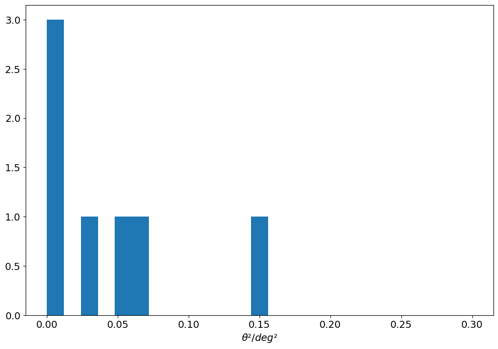
[30]:
theta = angular_separation(
    events["HillasReconstructor_az"].quantity,
    events["HillasReconstructor_alt"].quantity,
    events["true_az"].quantity,
    events["true_alt"].quantity,
)

plt.hist(theta.to_value(u.deg) ** 2, bins=25, range=[0, 0.3])
plt.xlabel(r"$\theta² / deg²$")
None
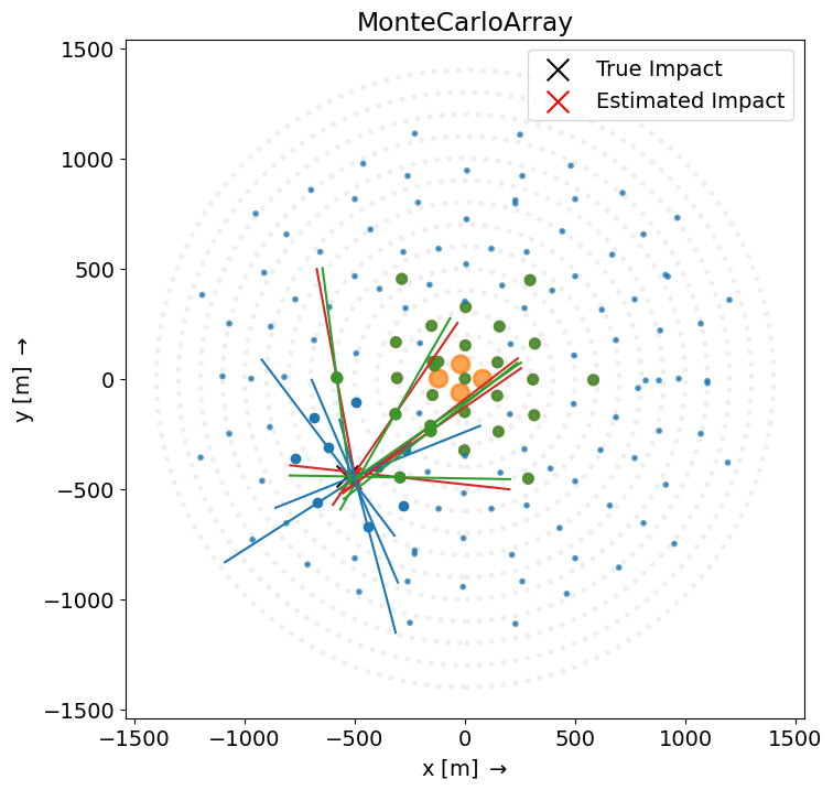
ArrayDisplay
[31]:
from ctapipe.visualization import ArrayDisplay


angle_offset = plotting_event.pointing.array_azimuth

plotting_hillas = {
    tel_id: dl1.parameters.hillas for tel_id, dl1 in plotting_event.dl1.tel.items()
}

plotting_core = {
    tel_id: dl1.parameters.core.psi for tel_id, dl1 in plotting_event.dl1.tel.items()
}


disp = ArrayDisplay(source.subarray)

disp.set_line_hillas(plotting_hillas, plotting_core, 500)

plt.scatter(
    plotting_event.simulation.shower.core_x,
    plotting_event.simulation.shower.core_y,
    s=200,
    c="k",
    marker="x",
    label="True Impact",
)
plt.scatter(
    plotting_event.dl2.stereo.geometry["HillasReconstructor"].core_x,
    plotting_event.dl2.stereo.geometry["HillasReconstructor"].core_y,
    s=200,
    c="r",
    marker="x",
    label="Estimated Impact",
)

plt.legend()
# plt.xlim(-400, 400)
# plt.ylim(-400, 400)
[31]:
<matplotlib.legend.Legend at 0x7f4124c90b50>
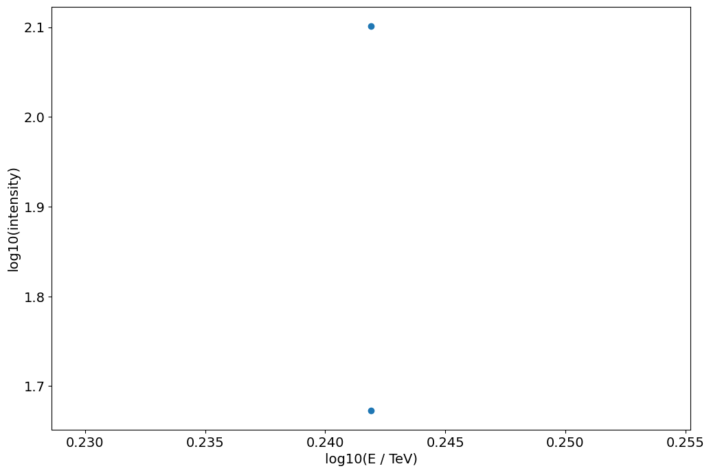
Reading the LST dl1 data
[32]:
loader = TableLoader(f.name, load_simulated=True, load_dl1_parameters=True)

dl1_table = loader.read_telescope_events(["LST_LST_LSTCam"])
[33]:
plt.scatter(
    np.log10(dl1_table["true_energy"].quantity / u.TeV),
    np.log10(dl1_table["hillas_intensity"]),
)
plt.xlabel("log10(E / TeV)")
plt.ylabel("log10(intensity)")
None
Isn’t python slow?
Many of you might have heard: “Python is slow”.
That’s trueish.
All python objects are classes living on the heap, even integers.
Looping over lots of “primitives” is quite slow compared to other languages.
But: “Premature Optimization is the root of all evil” — Donald Knuth
So profile to find exactly what is slow.
Why use python then?
Python works very well as glue for libraries of all kinds of languages
Python has a rich ecosystem for data science, physics, algorithms, astronomy
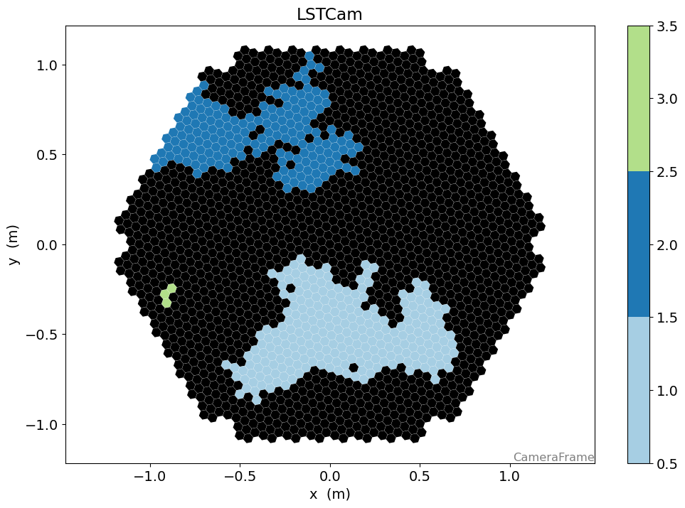
Example: Number of Islands
Find all groups of pixels, that survived the cleaning
[34]:
from ctapipe.image import toymodel
from ctapipe.instrument import SubarrayDescription


geometry = loader.subarray.tel[1].camera.geometry
Let’s create a toy images with several islands;
[35]:
np.random.seed(42)

image = np.zeros(geometry.n_pixels)


for i in range(9):

    model = toymodel.Gaussian(
        x=np.random.uniform(-0.8, 0.8) * u.m,
        y=np.random.uniform(-0.8, 0.8) * u.m,
        width=np.random.uniform(0.05, 0.075) * u.m,
        length=np.random.uniform(0.1, 0.15) * u.m,
        psi=np.random.uniform(0, 2 * np.pi) * u.rad,
    )

    new_image, sig, bg = model.generate_image(
        geometry, intensity=np.random.uniform(1000, 3000), nsb_level_pe=5
    )
    image += new_image
[36]:
clean = tailcuts_clean(
    geometry,
    image,
    picture_thresh=10,
    boundary_thresh=5,
    min_number_picture_neighbors=2,
)
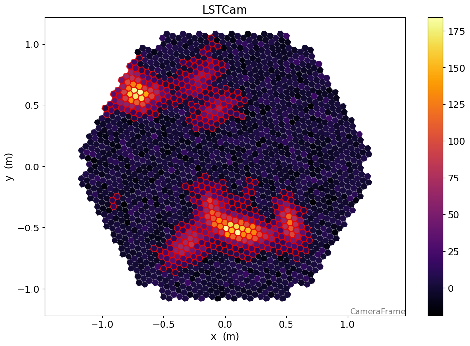
[37]:
disp = CameraDisplay(geometry)
disp.image = image
disp.highlight_pixels(clean, color="xkcd:red", linewidth=1.5)
disp.add_colorbar()
[38]:
def num_islands_python(camera, clean):
    """A breadth first search to find connected islands of neighboring pixels in the cleaning set"""

    # the camera geometry has a [n_pixel, n_pixel] boolean array
    # that is True where two pixels are neighbors
    neighbors = camera.neighbor_matrix

    island_ids = np.zeros(camera.n_pixels)
    current_island = 0

    # a set to remember which pixels we already visited
    visited = set()

    # go only through the pixels, that survived cleaning
    for pix_id in np.where(clean)[0]:
        if pix_id not in visited:
            # remember that we already checked this pixel
            visited.add(pix_id)

            # if we land in the outer loop again, we found a new island
            current_island += 1
            island_ids[pix_id] = current_island

            # now check all neighbors of the current pixel recursively
            to_check = set(np.where(neighbors[pix_id] & clean)[0])
            while to_check:
                pix_id = to_check.pop()

                if pix_id not in visited:
                    visited.add(pix_id)
                    island_ids[pix_id] = current_island

                    to_check.update(np.where(neighbors[pix_id] & clean)[0])

    n_islands = current_island
    return n_islands, island_ids
[39]:
n_islands, island_ids = num_islands_python(geometry, clean)
[40]:
from matplotlib.colors import ListedColormap

cmap = plt.get_cmap("Paired")
cmap = ListedColormap(cmap.colors[:n_islands])
cmap.set_under("k")

disp = CameraDisplay(geometry)
disp.image = island_ids
disp.cmap = cmap
disp.set_limits_minmax(0.5, n_islands + 0.5)
disp.add_colorbar()

[41]:
%timeit num_islands_python(geometry, clean)
2.42 ms ± 14.8 µs per loop (mean ± std. dev. of 7 runs, 100 loops each)
[42]:
from scipy.sparse.csgraph import connected_components


def num_islands_scipy(geometry, clean):
    neighbors = geometry.neighbor_matrix_sparse

    clean_neighbors = neighbors[clean][:, clean]
    num_islands, labels = connected_components(clean_neighbors, directed=False)

    island_ids = np.zeros(geometry.n_pixels)
    island_ids[clean] = labels + 1

    return num_islands, island_ids
[43]:
n_islands_s, island_ids_s = num_islands_scipy(geometry, clean)
[44]:
disp = CameraDisplay(geometry)
disp.image = island_ids_s
disp.cmap = cmap
disp.set_limits_minmax(0.5, n_islands_s + 0.5)
disp.add_colorbar()
[45]:
%timeit num_islands_scipy(geometry, clean)
566 µs ± 4.46 µs per loop (mean ± std. dev. of 7 runs, 1,000 loops each)
A lot less code, and a factor 3 speed improvement
Finally, current ctapipe implementation is using numba:
[46]:
%timeit number_of_islands(geometry, clean)
24.1 µs ± 160 ns per loop (mean ± std. dev. of 7 runs, 10,000 loops each)