2018 LST Bootcamp walkthrough
![]()
LST Analysis Bootcamp
Padova, 26.11.2018
Maximilian Nöthe (@maxnoe) & Kai A. Brügge (@mackaiver)
[1]:
import matplotlib.pyplot as plt
import numpy as np

%matplotlib inline
[2]:
plt.rcParams['figure.figsize'] = (12, 8)
plt.rcParams['font.size'] = 14
plt.rcParams['figure.figsize']
[2]:
[12.0, 8.0]
Table of Contents
General Information
Design
DL0 → DL3 analysis
Currently some R0 → DL0 code to be able to analyze simtel files
ctapipe is built upon the Scientific Python Stack, core dependencies are
numpy
scipy
astropy
Developement
ctapipe is developed as Open Source Software (Currently under MIT License) at https://github.com/cta-observatory/ctapipe
We use the “Github-Workflow”:
Few people (e.g. @kosack, @mackaiver) have write access to the main repository
Contributors fork the main repository and work on branches
Pull Requests are merged after Code Review and automatic execution of the test suite
Early developement stage ⇒ backwards-incompatible API changes might and will happen
Many open design questions ⇒ Core Developer Meeting in the second week of December in Dortmund
What’s there?
Reading simtel simulation files
Simple calibration, cleaning and feature extraction functions
Camera and Array plotting
Coordinate frames and transformations
Stereo-reconstruction using line intersections
What’s still missing?
Easy to use IO of analysis results to standard data formats (e.g. FITS, hdf5)
Easy to use “analysis builder”
A “Standard Analysis”
Good integration with machine learning techniques
IRF calculation
Defining APIs for IO, instrument description access etc.
Most code only tested on HESSIO simulations
Documentation, e.g. formal definitions of coordinate frames
What can you do?
Report issues
Hard to get started? Tell us where you are stuck
Tell user stories
Missing features
Start contributing
ctapipe needs more workpower
Implement new reconstruction features
A simple hillas analysis
Reading in simtel files
[3]:
from ctapipe.io import EventSource
from ctapipe.utils.datasets import get_dataset_path

input_url = get_dataset_path('gamma_test_large.simtel.gz')

# EventSource() automatically detects what kind of file we are giving it,
# if already supported by ctapipe
source = EventSource(input_url, max_events=49)

print(type(source))
<class 'ctapipe.io.simteleventsource.SimTelEventSource'>
[4]:
for event in source:
    print('Id: {}, E = {:1.3f}, Telescopes: {}'.format(event.count, event.simulation.shower.energy, len(event.r0.tel)))
Id: 0, E = 0.571 TeV, Telescopes: 4
Id: 1, E = 1.864 TeV, Telescopes: 9
Id: 2, E = 1.864 TeV, Telescopes: 4
Id: 3, E = 1.864 TeV, Telescopes: 17
Id: 4, E = 1.864 TeV, Telescopes: 2
Id: 5, E = 0.464 TeV, Telescopes: 7
Id: 6, E = 0.017 TeV, Telescopes: 2
Id: 7, E = 76.426 TeV, Telescopes: 4
Id: 8, E = 76.426 TeV, Telescopes: 16
Id: 9, E = 76.426 TeV, Telescopes: 3
Id: 10, E = 0.267 TeV, Telescopes: 5
Id: 11, E = 0.010 TeV, Telescopes: 2
Id: 12, E = 1.407 TeV, Telescopes: 3
Id: 13, E = 1.407 TeV, Telescopes: 3
Id: 14, E = 0.121 TeV, Telescopes: 10
Id: 15, E = 0.032 TeV, Telescopes: 4
Id: 16, E = 0.073 TeV, Telescopes: 2
Id: 17, E = 0.129 TeV, Telescopes: 3
Id: 18, E = 0.129 TeV, Telescopes: 2
Id: 19, E = 10.220 TeV, Telescopes: 2
Id: 20, E = 10.220 TeV, Telescopes: 4
Id: 21, E = 10.220 TeV, Telescopes: 4
Id: 22, E = 0.055 TeV, Telescopes: 2
Id: 23, E = 0.100 TeV, Telescopes: 3
Id: 24, E = 0.079 TeV, Telescopes: 5
Id: 25, E = 0.127 TeV, Telescopes: 7
Id: 26, E = 3.923 TeV, Telescopes: 4
Id: 27, E = 3.923 TeV, Telescopes: 2
Id: 28, E = 3.923 TeV, Telescopes: 4
Id: 29, E = 0.147 TeV, Telescopes: 6
Id: 30, E = 0.974 TeV, Telescopes: 6
Id: 31, E = 0.974 TeV, Telescopes: 3
Id: 32, E = 0.474 TeV, Telescopes: 4
Id: 33, E = 0.474 TeV, Telescopes: 4
Id: 34, E = 0.110 TeV, Telescopes: 2
Id: 35, E = 0.103 TeV, Telescopes: 2
Id: 36, E = 0.120 TeV, Telescopes: 4
Id: 37, E = 0.078 TeV, Telescopes: 4
Id: 38, E = 0.079 TeV, Telescopes: 2
Id: 39, E = 0.592 TeV, Telescopes: 4
Id: 40, E = 0.066 TeV, Telescopes: 6
Id: 41, E = 0.126 TeV, Telescopes: 3
Id: 42, E = 0.126 TeV, Telescopes: 2
Id: 43, E = 0.129 TeV, Telescopes: 2
Id: 44, E = 0.017 TeV, Telescopes: 3
Id: 45, E = 0.053 TeV, Telescopes: 2
Id: 46, E = 0.009 TeV, Telescopes: 2
Id: 47, E = 0.248 TeV, Telescopes: 4
Id: 48, E = 0.248 TeV, Telescopes: 11
Each event is a DataContainer holding several Fields of data, which can be containers or just numbers. Let’s look a one event:
[5]:
event
[5]:
ctapipe.containers.ArrayEventContainer:
                       index.*: event indexing information
                          r0.*: Raw Data
                          r1.*: R1 Calibrated Data
                         dl0.*: DL0 Data Volume Reduced Data
                         dl1.*: DL1 Calibrated image
                         dl2.*: DL2 reconstruction info
                  simulation.*: Simulated Event Information
                     trigger.*: central trigger information
                         count: number of events processed
                    pointing.*: Array and telescope pointing positions
                 calibration.*: Container for calibration coefficients for the
                                current event
                         mon.*: container for event-wise monitoring data (MON)
[6]:
source.subarray.camera_types
[6]:
[CameraDescription(camera_name=LSTCam, geometry=LSTCam, readout=LSTCam),
 CameraDescription(camera_name=ASTRICam, geometry=ASTRICam, readout=ASTRICam),
 CameraDescription(camera_name=FlashCam, geometry=FlashCam, readout=FlashCam)]
[7]:
len(event.r0.tel), len(event.r1.tel)
[7]:
(11, 11)
Data calibration
The CameraCalibrator calibrates the event (obtaining the dl1 images).
[8]:
from ctapipe.calib import CameraCalibrator

calibrator = CameraCalibrator(subarray=source.subarray)
[9]:
calibrator(event)
Event displays
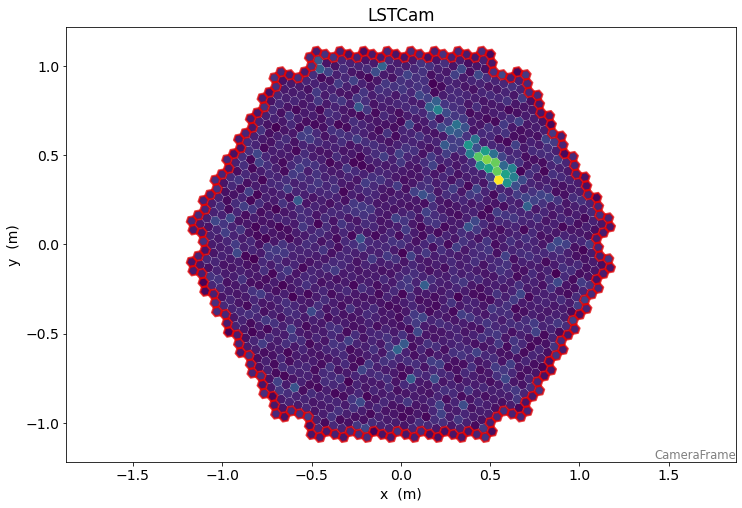
Let’s use ctapipe’s plotting facilities to plot the telescope images
[10]:
event.dl1.tel.keys()
[10]:
dict_keys([1, 2, 3, 4, 5, 7, 9, 11, 13, 16, 19])
[11]:
tel_id = 4
[12]:
geometry = source.subarray.tel[tel_id].camera.geometry
dl1 = event.dl1.tel[tel_id]

geometry, dl1
[12]:
(CameraGeometry(camera_name='LSTCam', pix_type=<PixelShape.HEXAGON: 'hexagon'>, npix=1855, cam_rot=0.0 deg, pix_rot=100.89299992867878 deg),
 ctapipe.containers.DL1CameraContainer:
                          image: Numpy array of camera image, after waveform
                                 extraction.Shape: (n_pixel) as a 1-D array with
                                 type float32
                      peak_time: Numpy array containing position of the peak of
                                 the pulse as determined by the extractor. Shape:
                                 (n_pixel, ) as a 1-D array with type float32
                     image_mask: Boolean numpy array where True means the pixel
                                 has passed cleaning. Shape: (n_pixel, ) as a 1-D
                                 array with type bool
                     parameters: Image parameters)
[13]:
dl1.image
[13]:
array([ 1.8977832 , -1.7927673 ,  1.8373003 , ..., -1.330724  ,
        1.0946255 ,  0.36395848], dtype=float32)
[14]:
from ctapipe.visualization import CameraDisplay

display = CameraDisplay(geometry)

# right now, there might be one image per gain channel.
# This will change as soon as
display.image = dl1.image
display.add_colorbar()
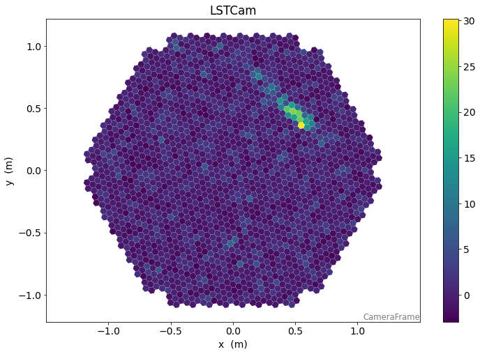
Image Cleaning
[15]:
from ctapipe.image.cleaning import tailcuts_clean
[16]:
# unoptimized cleaning levels, copied from
# https://github.com/tudo-astroparticlephysics/cta_preprocessing
cleaning_level = {
    'ASTRICam': (5, 7, 2),  # (5, 10)?
    'LSTCam': (3.5, 7.5, 2),  # ?? (3, 6) for Abelardo...
    'FlashCam': (4, 8, 2),  # there is some scaling missing?
}
[17]:
boundary, picture, min_neighbors = cleaning_level[geometry.camera_name]

clean = tailcuts_clean(
    geometry,
    dl1.image,
    boundary_thresh=boundary,
    picture_thresh=picture,
    min_number_picture_neighbors=min_neighbors
)
[18]:
fig, (ax1, ax2) = plt.subplots(1, 2, figsize=(15, 5))

d1 = CameraDisplay(geometry, ax=ax1)
d2 = CameraDisplay(geometry, ax=ax2)

ax1.set_title('Image')
d1.image = dl1.image
d1.add_colorbar(ax=ax1)

ax2.set_title('Pulse Time')
d2.image = dl1.peak_time - np.average(dl1.peak_time, weights=dl1.image)
d2.cmap = 'RdBu_r'
d2.add_colorbar(ax=ax2)
d2.set_limits_minmax(-20,20)

d1.highlight_pixels(clean, color='red', linewidth=1)
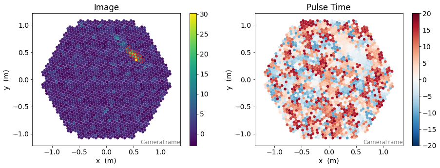
Image Parameters
[19]:
from ctapipe.image import hillas_parameters, leakage_parameters, concentration_parameters
from ctapipe.image import timing_parameters
from ctapipe.image import number_of_islands
from ctapipe.image import camera_to_shower_coordinates
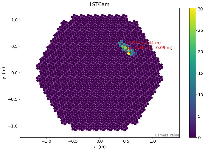
[20]:
hillas = hillas_parameters(geometry[clean], dl1.image[clean])

print(hillas)
{'intensity': 293.30156207084656,
 'kurtosis': 2.1156918832117624,
 'length': <Quantity 0.09458967 m>,
 'length_uncertainty': <Quantity 0.00291695 m>,
 'phi': <Angle 0.71440377 rad>,
 'psi': <Angle -0.71608044 rad>,
 'r': <Quantity 0.67893267 m>,
 'skewness': -0.15071029797454388,
 'width': <Quantity 0.03181493 m>,
 'width_uncertainty': <Quantity 0.00096868 m>,
 'x': <Quantity 0.51292278 m>,
 'y': <Quantity 0.44481435 m>}
[21]:
display = CameraDisplay(geometry)

# set "unclean" pixels to 0
cleaned = dl1.image.copy()
cleaned[~clean] = 0.0

display.image = cleaned
display.add_colorbar()

display.overlay_moments(hillas, color='xkcd:red')
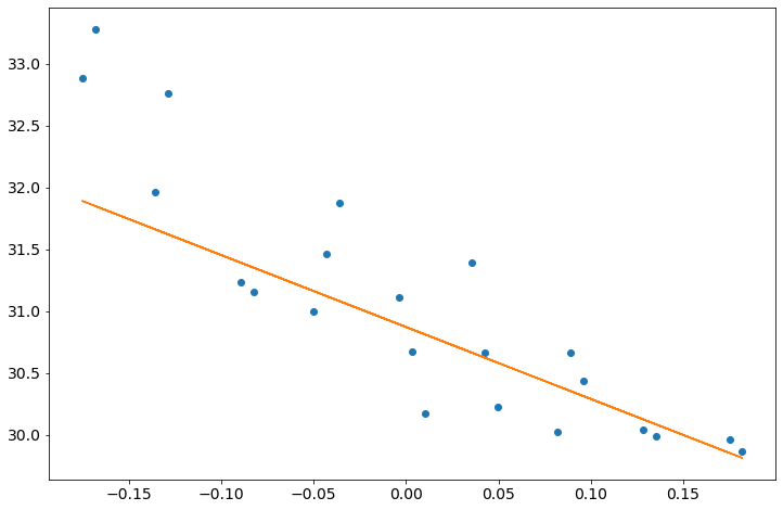
[22]:
timing = timing_parameters(
    geometry,
    dl1.image,
    dl1.peak_time,
    hillas,
    clean
)

print(timing)
{'deviation': 0.5507465160185104,
 'intercept': 30.871464798739247,
 'slope': <Quantity -5.81771647 1 / m>}
[23]:
long, trans = camera_to_shower_coordinates(
    geometry.pix_x, geometry.pix_y,hillas.x, hillas.y, hillas.psi
)

plt.plot(long[clean], dl1.peak_time[clean], 'o')
plt.plot(long[clean], timing.slope * long[clean] + timing.intercept)
[23]:
[<matplotlib.lines.Line2D at 0x7f33b7af2f70>]
[24]:
l = leakage_parameters(geometry, dl1.image, clean)
print(l)
{'intensity_width_1': 0.0,
 'intensity_width_2': 0.0,
 'pixels_width_1': 0.0,
 'pixels_width_2': 0.0}
[25]:
disp = CameraDisplay(geometry)
disp.image = dl1.image
disp.highlight_pixels(geometry.get_border_pixel_mask(1), linewidth=2, color='xkcd:red')
[26]:
n_islands, island_id = number_of_islands(geometry, clean)

print(n_islands)
1
[27]:
conc = concentration_parameters(geometry, dl1.image, hillas)
print(conc)
{'cog': 0.2901097326436822,
 'core': 0.34470898401576955,
 'pixel': 0.10290955973463788}
Putting it all together / Stereo reconstruction
[28]:
import astropy.units as u
from astropy.coordinates import SkyCoord, AltAz

from ctapipe.containers import ImageParametersContainer
from ctapipe.io import EventSource
from ctapipe.utils.datasets import get_dataset_path

from ctapipe.calib import CameraCalibrator

from ctapipe.image import tailcuts_clean, number_of_islands
from ctapipe.image import hillas_parameters, leakage_parameters, concentration_parameters
from ctapipe.image import timing_parameters

from ctapipe.reco import HillasReconstructor

from ctapipe.io import HDF5TableWriter

from copy import deepcopy
import tempfile

# unoptimized cleaning levels, copied from
# https://github.com/tudo-astroparticlephysics/cta_preprocessing
cleaning_level = {
    'ASTRICam': (5, 7, 2),  # (5, 10)?
    'LSTCam': (3.5, 7.5, 2),  # ?? (3, 6) for Abelardo...
    'FlashCam': (4, 8, 2),  # there is some scaling missing?
}


input_url = get_dataset_path('gamma_test_large.simtel.gz')
source = EventSource(input_url)

calibrator = CameraCalibrator(subarray=source.subarray)

horizon_frame = AltAz()

f = tempfile.NamedTemporaryFile(suffix='.hdf5')

with HDF5TableWriter(f.name, mode='w', group_name='events') as writer:

    for event in source:
        print('Id: {}, E = {:1.3f}, Telescopes: {}'.format(event.count, event.simulation.shower.energy, len(event.r0.tel)))

        calibrator(event)

        # mapping of telescope_id to parameters for stereo reconstruction
        hillas_containers = {}
        telescope_pointings = {}
        time_gradients = {}

        for telescope_id, dl1 in event.dl1.tel.items():

            # Initialize an empty container for DL1b data
            event.dl1.tel[telescope_id].parameters = ImageParametersContainer()

            geometry = source.subarray.tels[telescope_id].camera.geometry
            image = dl1.image
            peak_time = dl1.peak_time

            boundary, picture, min_neighbors = cleaning_level[geometry.camera_name]

            clean = tailcuts_clean(
                geometry,
                image,
                boundary_thresh=boundary,
                picture_thresh=picture,
                min_number_picture_neighbors=min_neighbors
            )

            # require more than five pixels after cleaning in each telescope
            if clean.sum() < 5:
                continue

            hillas_c = hillas_parameters(geometry[clean], image[clean])
            event.dl1.tel[telescope_id].parameters.hillas = hillas_c

            leakage_c = leakage_parameters(geometry, image, clean)
            n_islands, island_ids = number_of_islands(geometry, clean)

            # remove events with high leakage
            if leakage_c.intensity_width_2 > 0.2:
                continue

            timing_c = timing_parameters(geometry, image, peak_time, hillas_c, clean)

            hillas_containers[telescope_id] = hillas_c

            # ssts have no timing in prod3b, so we'll use the skewness
            time_gradients[telescope_id] = timing_c.slope.value if geometry.camera_name != 'ASTRICam' else hillas_c.skewness

            # this makes sure, that we get an arrow in the array plow for each telescope
            # might have the wrong direction though
            if abs(time_gradients[telescope_id]) < 0.2:
                time_gradients[telescope_id] = 1.0

            telescope_pointings[telescope_id] = SkyCoord(
                alt=event.pointing.tel[telescope_id].altitude,
                az=event.pointing.tel[telescope_id].azimuth,
                frame=horizon_frame
            )

        # the array pointing is needed for the creation of the TiltedFrame to perform the
        # impact point reconstruction
        array_pointing = SkyCoord(
            az=event.pointing.array_azimuth,
            alt=event.pointing.array_altitude,
            frame=horizon_frame
        )

        if len(hillas_containers) > 2:
            reco = HillasReconstructor(source.subarray)
            stereo = reco._predict(
                event,
                hillas_containers,
                source.subarray,
                array_pointing,
                telescope_pointings
            )

            writer.write('reconstructed', stereo)
            writer.write('true', event.simulation.shower)

            print('  Alt: {:.2f}°'.format(stereo.alt.deg))
            print('  Az: {:.2f}°'.format(stereo.az.deg))
            print('  Hmax: {:.0f}'.format(stereo.h_max))
            print('  CoreX: {:.1f}'.format(stereo.core_x))
            print('  CoreY: {:.1f}'.format(stereo.core_y))

        # save a nice event for plotting later
        if event.count == 3:

            core_dict = {
                tel_id: dl1.parameters.core.psi for tel_id, dl1 in event.dl1.tel.items()
            }
            plotting_core = core_dict
            plotting_event = deepcopy(event)
            plotting_hillas = hillas_containers
            plotting_timing = time_gradients
            plotting_stereo = stereo
Id: 0, E = 0.571 TeV, Telescopes: 4
Id: 1, E = 1.864 TeV, Telescopes: 9
Column tel_ids of container ReconstructedGeometryContainer in table reconstructed not writable, skipping
  Alt: 68.25°
  Az: -353.46°
  Hmax: 6798 m
  CoreX: -48.5 m
  CoreY: -394.6 m
Id: 2, E = 1.864 TeV, Telescopes: 4
  Alt: 68.49°
  Az: -354.35°
  Hmax: 7050 m
  CoreX: -419.5 m
  CoreY: -574.8 m
Id: 3, E = 1.864 TeV, Telescopes: 17
  Alt: 68.47°
  Az: -353.41°
  Hmax: 6655 m
  CoreX: 42.2 m
  CoreY: 67.4 m
Id: 4, E = 1.864 TeV, Telescopes: 2
Id: 5, E = 0.464 TeV, Telescopes: 7
  Alt: 71.92°
  Az: -1.07°
  Hmax: 8684 m
  CoreX: -66.1 m
  CoreY: 289.6 m
Id: 6, E = 0.017 TeV, Telescopes: 2
Id: 7, E = 76.426 TeV, Telescopes: 4
Id: 8, E = 76.426 TeV, Telescopes: 16
  Alt: 75.26°
  Az: -353.94°
  Hmax: 5815 m
  CoreX: 137.1 m
  CoreY: 449.8 m
Id: 9, E = 76.426 TeV, Telescopes: 3
  Alt: 74.99°
  Az: -354.03°
  Hmax: 7485 m
  CoreX: 913.0 m
  CoreY: -995.4 m
Id: 10, E = 0.267 TeV, Telescopes: 5
Id: 11, E = 0.010 TeV, Telescopes: 2
Id: 12, E = 1.407 TeV, Telescopes: 3
Id: 13, E = 1.407 TeV, Telescopes: 3
Id: 14, E = 0.121 TeV, Telescopes: 10
  Alt: 67.41°
  Az: -0.73°
  Hmax: 13016 m
  CoreX: -163.9 m
  CoreY: -137.2 m
Id: 15, E = 0.032 TeV, Telescopes: 4
  Alt: 71.91°
  Az: -0.47°
  Hmax: 7848 m
  CoreX: 21.2 m
  CoreY: 65.8 m
Id: 16, E = 0.073 TeV, Telescopes: 2
Id: 17, E = 0.129 TeV, Telescopes: 3
Id: 18, E = 0.129 TeV, Telescopes: 2
Id: 19, E = 10.220 TeV, Telescopes: 2
Id: 20, E = 10.220 TeV, Telescopes: 4
Id: 21, E = 10.220 TeV, Telescopes: 4
Id: 22, E = 0.055 TeV, Telescopes: 2
Id: 23, E = 0.100 TeV, Telescopes: 3
Id: 24, E = 0.079 TeV, Telescopes: 5
Id: 25, E = 0.127 TeV, Telescopes: 7
  Alt: 70.11°
  Az: -4.55°
  Hmax: 8605 m
  CoreX: 23.1 m
  CoreY: -198.6 m
Id: 26, E = 3.923 TeV, Telescopes: 4
Id: 27, E = 3.923 TeV, Telescopes: 2
Id: 28, E = 3.923 TeV, Telescopes: 4
Id: 29, E = 0.147 TeV, Telescopes: 6
  Alt: 70.10°
  Az: -3.79°
  Hmax: 5555 m
  CoreX: 131.2 m
  CoreY: 224.3 m
Id: 30, E = 0.974 TeV, Telescopes: 6
  Alt: 73.40°
  Az: -5.78°
  Hmax: 8489 m
  CoreX: 460.3 m
  CoreY: 328.2 m
Id: 31, E = 0.974 TeV, Telescopes: 3
Id: 32, E = 0.474 TeV, Telescopes: 4
  Alt: 70.06°
  Az: -10.68°
  Hmax: 7234 m
  CoreX: -123.8 m
  CoreY: -478.5 m
Id: 33, E = 0.474 TeV, Telescopes: 4
Id: 34, E = 0.110 TeV, Telescopes: 2
Id: 35, E = 0.103 TeV, Telescopes: 2
Id: 36, E = 0.120 TeV, Telescopes: 4
  Alt: 68.60°
  Az: -8.66°
  Hmax: 10768 m
  CoreX: 118.9 m
  CoreY: -206.3 m
Id: 37, E = 0.078 TeV, Telescopes: 4
  Alt: 68.58°
  Az: -355.25°
  Hmax: 9472 m
  CoreX: -170.6 m
  CoreY: -115.5 m
Id: 38, E = 0.079 TeV, Telescopes: 2
Id: 39, E = 0.592 TeV, Telescopes: 4
Id: 40, E = 0.066 TeV, Telescopes: 6
  Alt: 68.82°
  Az: -6.06°
  Hmax: 10677 m
  CoreX: 67.5 m
  CoreY: -14.0 m
Id: 41, E = 0.126 TeV, Telescopes: 3
  Alt: 71.57°
  Az: -355.17°
  Hmax: 7758 m
  CoreX: -210.1 m
  CoreY: -308.9 m
Id: 42, E = 0.126 TeV, Telescopes: 2
Id: 43, E = 0.129 TeV, Telescopes: 2
Id: 44, E = 0.017 TeV, Telescopes: 3
Id: 45, E = 0.053 TeV, Telescopes: 2
Id: 46, E = 0.009 TeV, Telescopes: 2
Id: 47, E = 0.248 TeV, Telescopes: 4
  Alt: 71.94°
  Az: -0.06°
  Hmax: 10458 m
  CoreX: 467.2 m
  CoreY: 96.6 m
Id: 48, E = 0.248 TeV, Telescopes: 11
  Alt: 71.98°
  Az: -359.96°
  Hmax: 10188 m
  CoreX: 8.3 m
  CoreY: -147.3 m
Id: 49, E = 0.248 TeV, Telescopes: 4
Id: 50, E = 5.327 TeV, Telescopes: 2
Id: 51, E = 5.327 TeV, Telescopes: 18
  Alt: 67.08°
  Az: -351.11°
  Hmax: 6521 m
  CoreX: -340.4 m
  CoreY: 145.5 m
Id: 52, E = 5.327 TeV, Telescopes: 2
Id: 53, E = 0.095 TeV, Telescopes: 2
Id: 54, E = 0.937 TeV, Telescopes: 2
Id: 55, E = 0.937 TeV, Telescopes: 2
Id: 56, E = 0.937 TeV, Telescopes: 4
Id: 57, E = 0.937 TeV, Telescopes: 2
Id: 58, E = 0.161 TeV, Telescopes: 2
Id: 59, E = 0.407 TeV, Telescopes: 14
  Alt: 69.64°
  Az: -8.06°
  Hmax: 9542 m
  CoreX: -76.2 m
  CoreY: -88.8 m
Id: 60, E = 0.037 TeV, Telescopes: 3
  Alt: 67.22°
  Az: -358.15°
  Hmax: 13977 m
  CoreX: -437.6 m
  CoreY: 51.7 m
Id: 61, E = 0.020 TeV, Telescopes: 4
  Alt: 70.55°
  Az: -0.70°
  Hmax: 9237 m
  CoreX: 1.8 m
  CoreY: 123.1 m
Id: 62, E = 2.364 TeV, Telescopes: 4
Id: 63, E = 0.710 TeV, Telescopes: 8
  Alt: 71.35°
  Az: -349.97°
  Hmax: 10258 m
  CoreX: 302.8 m
  CoreY: 222.5 m
Id: 64, E = 0.710 TeV, Telescopes: 2
Id: 65, E = 1.158 TeV, Telescopes: 2
Id: 66, E = 0.055 TeV, Telescopes: 5
  Alt: 69.85°
  Az: -356.16°
  Hmax: 8673 m
  CoreX: -13.5 m
  CoreY: 160.4 m
Id: 67, E = 0.032 TeV, Telescopes: 2
Id: 68, E = 0.232 TeV, Telescopes: 3
Id: 69, E = 0.232 TeV, Telescopes: 2
Id: 70, E = 22.299 TeV, Telescopes: 5
  Alt: 66.80°
  Az: -358.30°
  Hmax: 6775 m
  CoreX: 139.1 m
  CoreY: -855.5 m
Id: 71, E = 22.299 TeV, Telescopes: 12
  Alt: 63.74°
  Az: -356.20°
  Hmax: 7888 m
  CoreX: -170.7 m
  CoreY: 271.0 m
Id: 72, E = 0.118 TeV, Telescopes: 3
Id: 73, E = 0.118 TeV, Telescopes: 3
Id: 74, E = 0.118 TeV, Telescopes: 5
  Alt: 67.02°
  Az: -5.38°
  Hmax: 9031 m
  CoreX: -61.6 m
  CoreY: -336.3 m
Id: 75, E = 0.101 TeV, Telescopes: 2
Id: 76, E = 0.065 TeV, Telescopes: 2
Id: 77, E = 3.581 TeV, Telescopes: 2
Id: 78, E = 3.581 TeV, Telescopes: 5
  Alt: 71.11°
  Az: -350.72°
  Hmax: 8273 m
  CoreX: 188.4 m
  CoreY: -667.7 m
Id: 79, E = 0.768 TeV, Telescopes: 5
Id: 80, E = 0.290 TeV, Telescopes: 2
Id: 81, E = 0.060 TeV, Telescopes: 2
Id: 82, E = 2.967 TeV, Telescopes: 2
Id: 83, E = 2.967 TeV, Telescopes: 2
Id: 84, E = 0.142 TeV, Telescopes: 4
  Alt: 69.42°
  Az: -358.78°
  Hmax: 10535 m
  CoreX: -149.3 m
  CoreY: -367.3 m
Id: 85, E = 0.142 TeV, Telescopes: 2
Id: 86, E = 0.435 TeV, Telescopes: 2
Id: 87, E = 0.435 TeV, Telescopes: 2
Id: 88, E = 0.339 TeV, Telescopes: 4
Id: 89, E = 1.851 TeV, Telescopes: 4
  Alt: 69.58°
  Az: -2.82°
  Hmax: 7769 m
  CoreX: -879.3 m
  CoreY: 105.7 m
Id: 90, E = 1.851 TeV, Telescopes: 6
  Alt: 69.47°
  Az: -2.52°
  Hmax: 7770 m
  CoreX: -711.7 m
  CoreY: -250.7 m
Id: 91, E = 0.189 TeV, Telescopes: 11
  Alt: 70.61°
  Az: -3.62°
  Hmax: 8684 m
  CoreX: -51.5 m
  CoreY: -92.9 m
Id: 92, E = 0.037 TeV, Telescopes: 3
Id: 93, E = 1.620 TeV, Telescopes: 4
  Alt: 69.32°
  Az: -7.08°
  Hmax: 7291 m
  CoreX: -867.7 m
  CoreY: -195.8 m
Id: 94, E = 1.620 TeV, Telescopes: 2
Id: 95, E = 1.620 TeV, Telescopes: 3
Id: 96, E = 1.620 TeV, Telescopes: 3
  Alt: 69.27°
  Az: -7.34°
  Hmax: 8186 m
  CoreX: 93.0 m
  CoreY: 864.1 m
Id: 97, E = 1.620 TeV, Telescopes: 7
  Alt: 69.19°
  Az: -6.66°
  Hmax: 7739 m
  CoreX: 317.6 m
  CoreY: -596.2 m
Id: 98, E = 0.112 TeV, Telescopes: 3
Id: 99, E = 0.322 TeV, Telescopes: 2
Id: 100, E = 0.322 TeV, Telescopes: 10
  Alt: 69.43°
  Az: -0.75°
  Hmax: 7702 m
  CoreX: -178.2 m
  CoreY: -223.8 m
Id: 101, E = 6.104 TeV, Telescopes: 4
Id: 102, E = 0.245 TeV, Telescopes: 3
Id: 103, E = 0.636 TeV, Telescopes: 2
Id: 104, E = 0.636 TeV, Telescopes: 4
Id: 105, E = 1.824 TeV, Telescopes: 6
  Alt: 70.25°
  Az: -0.72°
  Hmax: 7238 m
  CoreX: -612.5 m
  CoreY: -411.4 m
Id: 106, E = 1.824 TeV, Telescopes: 2
Id: 107, E = 1.824 TeV, Telescopes: 3
  Alt: 70.19°
  Az: -0.60°
  Hmax: 6885 m
  CoreX: 822.3 m
  CoreY: -124.4 m
Id: 108, E = 0.538 TeV, Telescopes: 5
Id: 109, E = 0.538 TeV, Telescopes: 2
[29]:
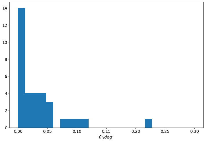
from astropy.coordinates.angle_utilities import angular_separation
import pandas as pd


df_rec = pd.read_hdf(f.name, key='events/reconstructed')
df_true = pd.read_hdf(f.name, key='events/true')


theta = angular_separation(
    df_rec.az.values * u.deg, df_rec.alt.values * u.deg,
    df_true.az.values * u.deg, df_true.alt.values * u.deg,
)

plt.hist(theta.to(u.deg).value**2, bins=25, range=[0, 0.3])
plt.xlabel(r'$\theta² / deg²$')
None
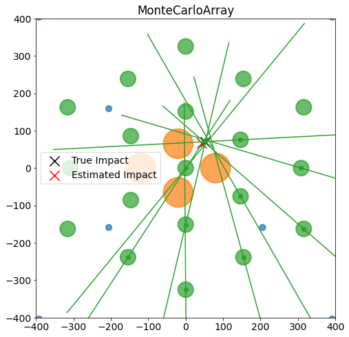
ArrayDisplay
[30]:
from ctapipe.visualization import ArrayDisplay


angle_offset = plotting_event.pointing.array_azimuth


disp = ArrayDisplay(source.subarray)

disp.set_line_hillas(plotting_hillas, plotting_core, 500)

plt.scatter(
    plotting_event.simulation.shower.core_x, plotting_event.simulation.shower.core_y,
    s=200, c='k', marker='x', label='True Impact',
)
plt.scatter(
    plotting_stereo.core_x, plotting_stereo.core_y,
    s=200, c='r', marker='x', label='Estimated Impact',
)

plt.legend()
plt.xlim(-400, 400)
plt.ylim(-400, 400)
[30]:
(-400.0, 400.0)
LST Mono with output
Let’s use the
HDF5TableWriterto save the dl1 Hillas parameter data to an hdf5 fileThis is not ideal yet and one of the major points to be discussed in two weeks
[31]:
from ctapipe.io import HDF5TableWriter
from ctapipe.core.container import Container, Field

input_url = get_dataset_path('gamma_test_large.simtel.gz')

source = EventSource(
    input_url,
    allowed_tels=[1, 2, 3, 4], # only use the first LST
)

calibrator = CameraCalibrator(subarray=source.subarray)

class EventInfo(Container):
    event_id = Field('event_id')
    obs_id =  Field('obs_id')
    telescope_id = Field('telescope_id')


with HDF5TableWriter(filename='hillas.h5', group_name='dl1', mode='w') as writer:

    for event in source:
        print('Id: {}, E = {:1.3f}, Telescopes: {}'.format(event.count, event.simulation.shower.energy, len(event.r0.tel)))

        calibrator(event)

        for telescope_id, dl1 in event.dl1.tel.items():

            geometry = source.subarray.tels[telescope_id].camera.geometry
            image = dl1.image
            peak_time = dl1.peak_time

            boundary, picture, min_neighbors = cleaning_level[geometry.camera_name]

            clean = tailcuts_clean(
                geometry,
                image,
                boundary_thresh=boundary,
                picture_thresh=picture,
                min_number_picture_neighbors=min_neighbors
            )

            if clean.sum() < 5:
                continue

            event_info = EventInfo(event_id=event.index.event_id, obs_id=event.index.obs_id, telescope_id=telescope_id)
            hillas_c = hillas_parameters(geometry[clean], image[clean])
            leakage_c = leakage_parameters(geometry, image, clean)
            timing_c = timing_parameters(geometry, image, peak_time, hillas_c, clean)

            writer.write('events', [event_info, event.simulation.shower, hillas_c, leakage_c, timing_c])
Id: 0, E = 1.864 TeV, Telescopes: 2
Id: 1, E = 0.017 TeV, Telescopes: 2
Id: 2, E = 0.010 TeV, Telescopes: 2
Id: 3, E = 0.121 TeV, Telescopes: 4
Id: 4, E = 0.032 TeV, Telescopes: 3
Id: 5, E = 0.073 TeV, Telescopes: 1
Id: 6, E = 0.129 TeV, Telescopes: 1
Id: 7, E = 0.079 TeV, Telescopes: 2
Id: 8, E = 0.127 TeV, Telescopes: 3
Id: 9, E = 0.147 TeV, Telescopes: 1
Id: 10, E = 0.103 TeV, Telescopes: 1
Id: 11, E = 0.078 TeV, Telescopes: 1
Id: 12, E = 0.592 TeV, Telescopes: 1
Id: 13, E = 0.066 TeV, Telescopes: 2
Id: 14, E = 0.017 TeV, Telescopes: 3
Id: 15, E = 0.009 TeV, Telescopes: 2
Id: 16, E = 0.248 TeV, Telescopes: 4
Id: 17, E = 5.327 TeV, Telescopes: 3
Id: 18, E = 0.407 TeV, Telescopes: 4
Id: 19, E = 0.037 TeV, Telescopes: 3
Id: 20, E = 0.020 TeV, Telescopes: 4
Id: 21, E = 0.710 TeV, Telescopes: 3
Id: 22, E = 0.055 TeV, Telescopes: 2
Id: 23, E = 0.032 TeV, Telescopes: 2
Id: 24, E = 0.118 TeV, Telescopes: 1
Id: 25, E = 0.142 TeV, Telescopes: 1
Id: 26, E = 0.189 TeV, Telescopes: 4
Id: 27, E = 0.037 TeV, Telescopes: 3
Id: 28, E = 0.112 TeV, Telescopes: 1
Id: 29, E = 0.322 TeV, Telescopes: 4
[32]:
import pandas as pd

df = pd.read_hdf('hillas.h5', key='dl1/events')
df.set_index(['obs_id', 'event_id', 'telescope_id'], inplace=True)
df.head()
[32]:
| energy | alt | az | core_x | core_y | h_first_int | x_max | shower_primary_id | intensity | skewness | ... | width | width_uncertainty | psi | pixels_width_1 | pixels_width_2 | intensity_width_1 | intensity_width_2 | intercept | deviation | slope | |||
|---|---|---|---|---|---|---|---|---|---|---|---|---|---|---|---|---|---|---|---|---|---|---|---|
| obs_id | event_id | telescope_id | |||||||||||||||||||||
| 7514 | 31012 | 2 | 1.863750 | 68.478978 | 6.384091 | 51.675117 | 69.654037 | 18171.726562 | 379.538452 | 0 | 475.328943 | 0.229954 | ... | 0.044190 | 0.001732 | 61.214904 | 0.011321 | 0.017790 | 0.651719 | 0.862295 | 32.153018 | 0.736568 | -5.222865 |
| 3 | 1.863750 | 68.478978 | 6.384091 | 51.675117 | 69.654037 | 18171.726562 | 379.538452 | 0 | 24086.055072 | 1.562733 | ... | 0.079858 | 0.000589 | -75.490119 | 0.009164 | 0.019407 | 0.114085 | 0.272478 | 33.675530 | 0.601674 | 1.950663 | ||
| 90914 | 2 | 0.016544 | 70.676229 | 3.107417 | -113.833435 | -142.343872 | 15776.052734 | 184.545456 | 0 | 78.789463 | -0.056639 | ... | 0.017989 | 0.001252 | 51.701246 | 0.000000 | 0.000000 | 0.000000 | 0.000000 | 30.751439 | 0.251867 | 1.631848 | |
| 4 | 0.016544 | 70.676229 | 3.107417 | -113.833435 | -142.343872 | 15776.052734 | 184.545456 | 0 | 110.688694 | 0.050001 | ... | 0.024432 | 0.001362 | 82.347736 | 0.000000 | 0.000000 | 0.000000 | 0.000000 | 30.185566 | 0.492260 | -2.437174 | ||
| 153614 | 1 | 0.010250 | 68.949967 | 2.666187 | -51.531204 | -106.752579 | 19824.572266 | 241.111115 | 0 | 76.273210 | -0.310947 | ... | 0.020285 | 0.001322 | 73.286384 | 0.000000 | 0.000000 | 0.000000 | 0.000000 | 30.057657 | 0.185710 | -2.750752 |
5 rows × 27 columns
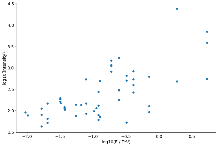
[33]:
plt.scatter(np.log10(df.energy), np.log10(df.intensity))
plt.xlabel('log10(E / TeV)')
plt.ylabel('log10(intensity)')
None
Isn’t python slow?
Many of you might have heard: “Python is slow”.
That’s trueish.
All python objects are classes living on the heap, event integers.
Looping over lots of “primitives” is quite slow compared to other languages.
But: “Premature Optimization is the root of all evil” — Donald Knuth
So profile to find exactly what is slow.
Why use python then?
Python works very well as glue for libraries of all kinds of languages
Python has a rich ecosystem for data science, physics, algorithms, astronomy
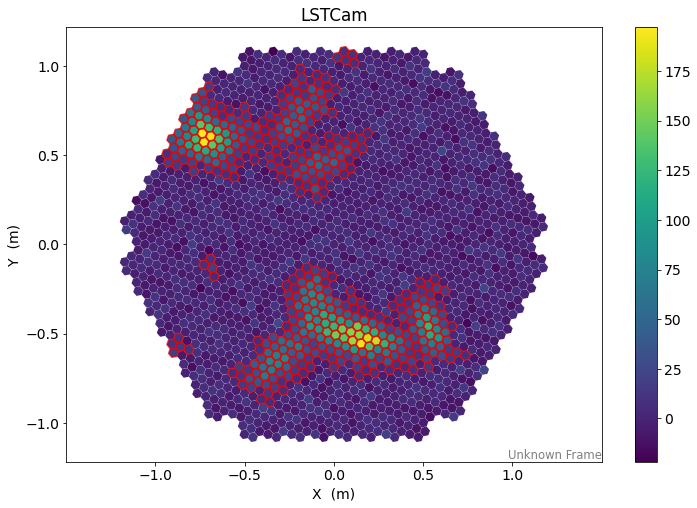
Example: Number of Islands
Find all groups of pixels, that survived the cleaning
[34]:
from ctapipe.image import toymodel
from ctapipe.instrument import CameraGeometry


geometry = CameraGeometry.from_name('LSTCam')
Let’s create a toy images with several islands;
[35]:
np.random.seed(42)

image = np.zeros(geometry.n_pixels)


for i in range(9):

    model = toymodel.Gaussian(
        x=np.random.uniform(-0.8, 0.8) * u.m,
        y=np.random.uniform(-0.8, 0.8) * u.m,
        width=np.random.uniform(0.05, 0.075) * u.m,
        length=np.random.uniform(0.1, 0.15) * u.m,
        psi=np.random.uniform(0, 2 * np.pi) * u.rad,
    )

    new_image, sig, bg = model.generate_image(
        geometry,
        intensity=np.random.uniform(1000, 3000),
        nsb_level_pe=5
    )
    image += new_image
[36]:
clean = tailcuts_clean(geometry, image, picture_thresh=10, boundary_thresh=5, min_number_picture_neighbors=2)
[37]:
disp = CameraDisplay(geometry)
disp.image = image
disp.highlight_pixels(clean, color='xkcd:red', linewidth=1.5)
disp.add_colorbar()
[38]:
def num_islands_python(camera, clean):
    ''' A breadth first search to find connected islands of neighboring pixels in the cleaning set'''

    # the camera geometry has a [n_pixel, n_pixel] boolean array
    # that is True where two pixels are neighbors
    neighbors = camera.neighbor_matrix

    island_ids = np.zeros(camera.n_pixels)
    current_island = 0

    # a set to remember which pixels we already visited
    visited = set()

    # go only through the pixels, that survived cleaning
    for pix_id in np.where(clean)[0]:
        if pix_id not in visited:
            # remember that we already checked this pixel
            visited.add(pix_id)

            # if we land in the outer loop again, we found a new island
            current_island += 1
            island_ids[pix_id] = current_island

            # now check all neighbors of the current pixel recursively
            to_check = set(np.where(neighbors[pix_id] & clean)[0])
            while to_check:
                pix_id = to_check.pop()

                if pix_id not in visited:
                    visited.add(pix_id)
                    island_ids[pix_id] = current_island

                    to_check.update(np.where(neighbors[pix_id] & clean)[0])

    n_islands = current_island
    return n_islands, island_ids
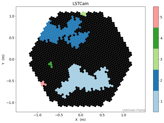
[39]:
n_islands, island_ids = num_islands_python(geometry, clean)
[40]:
from matplotlib.colors import ListedColormap

cmap = plt.get_cmap('Paired')
cmap = ListedColormap(cmap.colors[:n_islands])
cmap.set_under('k')

disp = CameraDisplay(geometry)
disp.image = island_ids
disp.cmap = cmap
disp.set_limits_minmax(0.5, n_islands + 0.5)
disp.add_colorbar()

[41]:
%timeit num_islands_python(geometry, clean)
2.22 ms ± 6.1 µs per loop (mean ± std. dev. of 7 runs, 100 loops each)
[42]:
from scipy.sparse.csgraph import connected_components

def num_islands_scipy(geometry, clean):
    neighbors = geometry.neighbor_matrix_sparse

    clean_neighbors = neighbors[clean][:, clean]
    num_islands, labels = connected_components(clean_neighbors, directed=False)

    island_ids = np.zeros(geometry.n_pixels)
    island_ids[clean] = labels + 1

    return num_islands, island_ids
[43]:
n_islands_s, island_ids_s = num_islands_scipy(geometry, clean)
[44]:
disp = CameraDisplay(geometry)
disp.image = island_ids_s
disp.cmap = cmap
disp.set_limits_minmax(0.5, n_islands_s + 0.5)
disp.add_colorbar()
[45]:
%timeit num_islands_scipy(geometry, clean)
438 µs ± 1.8 µs per loop (mean ± std. dev. of 7 runs, 1,000 loops each)
A lot less code, and a factor 3 speed improvement