Getting Started with ctapipe¶

This hands-on was presented at the Paris CTA Consoritum meeting (K. Kosack)

Part 1: load and loop over data¶

[1]:

from ctapipe.io import EventSource
from ctapipe import utils
from matplotlib import pyplot as plt
import numpy as np
%matplotlib inline

[2]:

path = utils.get_dataset_path("gamma_test_large.simtel.gz")

[3]:

source = EventSource(path, max_events=4)

for event in source:
    print(event.count, event.index.event_id, event.simulation.shower.energy)

0 23703 0.5707105398178101 TeV
1 31007 1.8637498617172241 TeV
2 31010 1.8637498617172241 TeV
3 31012 1.8637498617172241 TeV

[4]:

event

[4]:

ctapipe.containers.ArrayEventContainer:
                       index.*: event indexing information
                          r0.*: Raw Data
                          r1.*: R1 Calibrated Data
                         dl0.*: DL0 Data Volume Reduced Data
                         dl1.*: DL1 Calibrated image
                         dl2.*: DL2 reconstruction info
                  simulation.*: Simulated Event Information
                     trigger.*: central trigger information
                         count: number of events processed
                    pointing.*: Array and telescope pointing positions
                 calibration.*: Container for calibration coefficients for the
                                current event
                         mon.*: container for event-wise monitoring data (MON)

[5]:

event.r0

[5]:

ctapipe.containers.R0Container:
                        tel[*]: map of tel_id to R0CameraContainer

[6]:

for event in EventSource(path, max_events=4):
    print(event.count, event.r0.tel.keys())

0 dict_keys([13, 21, 25, 34])
1 dict_keys([7, 13, 16, 19, 25, 28, 34, 36, 42])
2 dict_keys([28, 46, 58, 68])
3 dict_keys([2, 3, 5, 6, 7, 8, 9, 10, 11, 12, 13, 14, 16, 18, 19, 20, 21])

[7]:

event.r0.tel[2]

[7]:

ctapipe.containers.R0CameraContainer:
                      waveform: numpy array containing ADC samples(n_channels,
                                n_pixels, n_samples)

[8]:

r0tel = event.r0.tel[3]

[9]:

r0tel.waveform

[9]:

array([[[267, 288, 286, ..., 297, 298, 312],
        [293, 285, 258, ..., 344, 373, 365],
        [333, 319, 289, ..., 306, 272, 261],
        ...,
        [255, 261, 270, ..., 258, 269, 271],
        [277, 312, 277, ..., 294, 323, 376],
        [319, 300, 347, ..., 283, 302, 265]],

       [[295, 304, 299, ..., 299, 298, 299],
        [298, 297, 300, ..., 300, 307, 304],
        [301, 305, 300, ..., 303, 300, 297],
        ...,
        [297, 296, 301, ..., 295, 297, 298],
        [295, 301, 296, ..., 300, 305, 302],
        [298, 300, 302, ..., 302, 297, 301]]], dtype=uint16)

[10]:

r0tel.waveform.shape

[10]:

(2, 1855, 30)

note that this is ($N_{channels}$, $N_{pixels}$, $N_{samples}$)

[11]:

plt.pcolormesh(r0tel.waveform[0])

[11]:

<matplotlib.collections.QuadMesh at 0x7f3b33f2a940>

../_images/tutorials_ctapipe_handson_13_1.png

[12]:

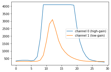
brightest_pixel = np.argmax(r0tel.waveform[0].sum(axis=1))
print(f"pixel {brightest_pixel} has sum {r0tel.waveform[0,1535].sum()}")

pixel 344 has sum 8642

[13]:

plt.plot(r0tel.waveform[0,brightest_pixel], label="channel 0 (high-gain)")
plt.plot(r0tel.waveform[1,brightest_pixel], label="channel 1 (low-gain)")
plt.legend()

[13]:

<matplotlib.legend.Legend at 0x7f3b33db04c0>

../_images/tutorials_ctapipe_handson_15_1.png

[14]:

from ipywidgets import interact

@interact
def view_waveform(chan=0, pix_id=brightest_pixel):
    plt.plot(r0tel.waveform[chan, pix_id])

try making this compare 2 waveforms

Part 2: Explore the instrument description¶

This is all well and good, but we don’t really know what camera or telescope this is… how do we get instrumental description info?

Currently this is returned inside the event (it will soon change to be separate in next version or so)

[15]:

subarray = source.subarray

[16]:

subarray

[16]:

SubarrayDescription(name='MonteCarloArray', num_tels=98)

[17]:

subarray.peek()

../_images/tutorials_ctapipe_handson_21_0.png

[18]:

subarray.to_table()

[18]:

Table length=98

tel_id	pos_x	pos_y	pos_z	name	type	camera_type	camera_index	optics_index	tel_description
	m	m	m
int16	float64	float64	float64	str5	str3	str8	int64	int64	str18
1	-20.0	65.0	16.0	LST	LST	LSTCam	2	2	LST_LST_LSTCam
2	-20.0	-65.0	16.0	LST	LST	LSTCam	2	2	LST_LST_LSTCam
3	80.0	0.0	16.0	LST	LST	LSTCam	2	2	LST_LST_LSTCam
4	-120.0	0.0	16.0	LST	LST	LSTCam	2	2	LST_LST_LSTCam
5	0.0	0.0	10.0	MST	MST	FlashCam	1	0	MST_MST_FlashCam
6	0.0	151.1999969482422	10.0	MST	MST	FlashCam	1	0	MST_MST_FlashCam
7	0.0	-151.1999969482422	10.0	MST	MST	FlashCam	1	0	MST_MST_FlashCam
8	146.65599060058594	75.5999984741211	10.0	MST	MST	FlashCam	1	0	MST_MST_FlashCam
9	146.65599060058594	-75.5999984741211	10.0	MST	MST	FlashCam	1	0	MST_MST_FlashCam
...	...	...	...	...	...	...	...	...	...
89	956.7870483398438	739.822998046875	5.0	ASTRI	SST	ASTRICam	0	1	SST_ASTRI_ASTRICam
90	956.7870483398438	-739.822998046875	5.0	ASTRI	SST	ASTRICam	0	1	SST_ASTRI_ASTRICam
91	-239.19699096679688	1109.7349853515625	5.0	ASTRI	SST	ASTRICam	0	1	SST_ASTRI_ASTRICam
92	-239.19699096679688	-1109.7349853515625	5.0	ASTRI	SST	ASTRICam	0	1	SST_ASTRI_ASTRICam
93	-956.7870483398438	739.822998046875	5.0	ASTRI	SST	ASTRICam	0	1	SST_ASTRI_ASTRICam
94	-956.7870483398438	-739.822998046875	5.0	ASTRI	SST	ASTRICam	0	1	SST_ASTRI_ASTRICam
95	1195.9840087890625	369.9119873046875	5.0	ASTRI	SST	ASTRICam	0	1	SST_ASTRI_ASTRICam
96	1195.9840087890625	-369.9119873046875	5.0	ASTRI	SST	ASTRICam	0	1	SST_ASTRI_ASTRICam
97	-1195.9840087890625	369.9119873046875	5.0	ASTRI	SST	ASTRICam	0	1	SST_ASTRI_ASTRICam
98	-1195.9840087890625	-369.9119873046875	5.0	ASTRI	SST	ASTRICam	0	1	SST_ASTRI_ASTRICam

[19]:

subarray.tel[2]

[19]:

TelescopeDescription(type=LST, name=LST, optics=LST, camera=LSTCam)

[20]:

subarray.tel[2].camera

[20]:

CameraDescription(camera_name=LSTCam, geometry=LSTCam, readout=LSTCam)

[21]:

subarray.tel[2].optics

[21]:

OpticsDescription(name=LST, equivalent_focal_length=28.00 m, num_mirrors=1, mirror_area=386.73 m2)

[22]:

tel = subarray.tel[2]

[23]:

tel.camera

[23]:

CameraDescription(camera_name=LSTCam, geometry=LSTCam, readout=LSTCam)

[24]:

tel.optics

[24]:

OpticsDescription(name=LST, equivalent_focal_length=28.00 m, num_mirrors=1, mirror_area=386.73 m2)

[25]:

tel.camera.geometry.pix_x

[25]:

$[0,~-0.0094487737,~-0.047244198,~\dots,~-0.6519913,~-0.6141959,~-0.62364468] \; \mathrm{m}$

[26]:

tel.camera.geometry.to_table()

[26]:

Table length=1855

pix_id	pix_x	pix_y	pix_area
	m	m	m2
int64	float64	float64	float64
0	0.0	0.0	0.002079326892271638
1	-0.00944877371419763	0.049099091130118636	0.002079326892271638
2	-0.04724419824666762	0.01636690782283136	0.002079326892271638
3	-0.037795424532469986	-0.03273218330728728	0.002079326892271638
4	0.00944877371419763	-0.049099091130118636	0.002079326892271638
5	0.04724419824666762	-0.01636690782283136	0.002079326892271638
6	0.037795424532469986	0.03273218330728728	0.002079326892271638
7	0.06614174532306863	-0.11456508825398498	0.002079326892271638
8	0.056692972312859496	-0.06546600078203366	0.002079326892271638
...	...	...	...
1845	-0.71814285557966	-0.8510456772325419	0.002079326892271638
1846	-0.6803376189247268	-0.8183116303101989	0.002079326892271638
1847	-0.6897863947508899	-0.7692125282055784	0.002079326892271638
1848	-0.6614400785362163	-0.9165097759887632	0.002079326892271638
1849	-0.6708888430985637	-0.8674107324148195	0.002079326892271638
1850	-0.7086940797534969	-0.9001447793371624	0.002079326892271638
1851	-0.6992453039273338	-0.949243881441783	0.002079326892271638
1852	-0.6519913027100532	-0.9656088780933837	0.002079326892271638
1853	-0.6141958992088292	-0.9328767234921034	0.002079326892271638
1854	-0.6236446750349923	-0.8837776213874828	0.002079326892271638

[27]:

tel.optics.mirror_area

[27]:

$386.73325 \; \mathrm{m^{2}}$

[28]:

from ctapipe.visualization import CameraDisplay

[29]:

disp = CameraDisplay(tel.camera.geometry)

../_images/tutorials_ctapipe_handson_33_0.png

[30]:

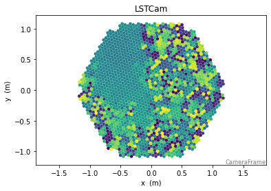
disp = CameraDisplay(tel.camera.geometry)
disp.image = r0tel.waveform[0,:,10]  # display channel 0, sample 0 (try others like 10)

../_images/tutorials_ctapipe_handson_34_0.png

** aside: ** show demo using a CameraDisplay in interactive mode in ipython rather than notebook

Part 3: Apply some calibration and trace integration¶

[31]:

from ctapipe.calib import CameraCalibrator

[32]:

calib = CameraCalibrator(subarray=subarray)

[33]:

for event in EventSource(path, max_events=4):
    calib(event) # fills in r1, dl0, and dl1
    print(event.dl1.tel.keys())

dict_keys([13, 21, 25, 34])
dict_keys([7, 13, 16, 19, 25, 28, 34, 36, 42])
dict_keys([28, 46, 58, 68])
dict_keys([2, 3, 5, 6, 7, 8, 9, 10, 11, 12, 13, 14, 16, 18, 19, 20, 21])

[34]:

event.dl1.tel[3]

[34]:

ctapipe.containers.DL1CameraContainer:
                         image: Numpy array of camera image, after waveform
                                extraction.Shape: (n_pixel) as a 1-D array with
                                type float32
                     peak_time: Numpy array containing position of the peak of
                                the pulse as determined by the extractor. Shape:
                                (n_pixel, ) as a 1-D array with type float32
                    image_mask: Boolean numpy array where True means the pixel
                                has passed cleaning. Shape: (n_pixel, ) as a 1-D
                                array with type bool
                    parameters: Image parameters

[35]:

dl1tel = event.dl1.tel[3]

[36]:

dl1tel.image.shape # note this will be gain-selected in next version, so will be just 1D array of 1855

[36]:

(1855,)

[37]:

dl1tel.peak_time

[37]:

array([34.26634 , 49.123714, 37.32338 , ..., 50.50625 , 45.477562,
       42.10054 ], dtype=float32)

[38]:

CameraDisplay(tel.camera.geometry, image=dl1tel.image)

[38]:

<ctapipe.visualization.mpl_camera.CameraDisplay at 0x7f3b2aa83370>

../_images/tutorials_ctapipe_handson_44_1.png

[39]:

CameraDisplay(tel.camera.geometry, image=dl1tel.peak_time)

[39]:

<ctapipe.visualization.mpl_camera.CameraDisplay at 0x7f3b2a8297f0>

../_images/tutorials_ctapipe_handson_45_1.png

Now for Hillas Parameters

[40]:

from ctapipe.image import hillas_parameters, tailcuts_clean

[41]:

image = dl1tel.image
mask = tailcuts_clean(tel.camera.geometry, image, picture_thresh=10, boundary_thresh=5)
mask

[41]:

array([False, False, False, ..., False, False, False])

[42]:

CameraDisplay(tel.camera.geometry, image=mask)

[42]:

<ctapipe.visualization.mpl_camera.CameraDisplay at 0x7f3b2a796a90>

../_images/tutorials_ctapipe_handson_49_1.png

[43]:

cleaned = image.copy()
cleaned[~mask] = 0

[44]:

disp = CameraDisplay(tel.camera.geometry, image=cleaned)
disp.cmap = plt.cm.coolwarm
disp.add_colorbar()
plt.xlim(-1.0,0)
plt.ylim(0,1.0)

[44]:

(0.0, 1.0)

../_images/tutorials_ctapipe_handson_51_1.png

[45]:

params = hillas_parameters(tel.camera.geometry, cleaned)
print(params)

{'intensity': 24075.39680337906,
 'kurtosis': 6.097240958638258,
 'length': <Quantity 0.20667421 m>,
 'length_uncertainty': <Quantity 0.00150362 m>,
 'phi': <Angle 2.23935833 rad>,
 'psi': <Angle -1.32341913 rad>,
 'r': <Quantity 0.92739417 m>,
 'skewness': 1.602462697612408,
 'width': <Quantity 0.07996111 m>,
 'width_uncertainty': <Quantity 0.00059966 m>,
 'x': <Quantity -0.57485289 m>,
 'y': <Quantity 0.72773903 m>}

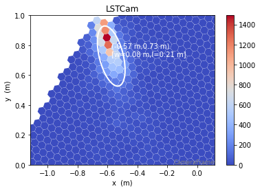
[46]:

disp = CameraDisplay(tel.camera.geometry, image=cleaned)
disp.cmap = plt.cm.coolwarm
disp.add_colorbar()
plt.xlim(-1.0,0)
plt.ylim(0,1.0)
disp.overlay_moments(params, color='white', lw=2)

../_images/tutorials_ctapipe_handson_53_0.png

Part 4: Let’s put it all together:¶

loop over events, selecting only telescopes of the same type (e.g. LST:LSTCam)
for each event, apply calibration/trace integration
calculate Hillas parameters
write out all hillas paremeters to a file that can be loaded with Pandas

first let’s select only those telescopes with LST:LSTCam

[47]:

subarray.telescope_types

[47]:

[TelescopeDescription(type=MST, name=MST, optics=MST, camera=FlashCam),
 TelescopeDescription(type=SST, name=ASTRI, optics=ASTRI, camera=ASTRICam),
 TelescopeDescription(type=LST, name=LST, optics=LST, camera=LSTCam)]

[48]:

subarray.get_tel_ids_for_type("LST_LST_LSTCam")

[48]:

[1, 2, 3, 4]

Now let’s write out program

[49]:

data = utils.get_dataset_path("gamma_test_large.simtel.gz")
source = EventSource(data, allowed_tels=[1,2,3,4],  max_events=10) # remove the max_events limit to get more stats

[50]:

for event in source:
    calib(event)

    for tel_id, tel_data in event.dl1.tel.items():
        tel = source.subarray.tel[tel_id]
        mask = tailcuts_clean(tel.camera.geometry, tel_data.image)
        params = hillas_parameters(tel.camera.geometry[mask], tel_data.image[mask])

[51]:

from ctapipe.io import HDF5TableWriter

[52]:

with HDF5TableWriter(filename='hillas.h5', group_name='dl1', overwrite=True) as writer:

    source = EventSource(data, allowed_tels=[1,2,3,4],  max_events=10)
    for event in source:
        calib(event)

        for tel_id, tel_data in event.dl1.tel.items():
            tel = source.subarray.tel[tel_id]
            mask = tailcuts_clean(tel.camera.geometry, tel_data.image)
            params = hillas_parameters(tel.camera.geometry[mask], tel_data.image[mask])
            writer.write("hillas", params)

We can now load in the file we created and plot it¶

[53]:

!ls *.h5

hillas.h5

[54]:

import pandas as pd

hillas = pd.read_hdf("hillas.h5", key='/dl1/hillas')
hillas

[54]:

	intensity	skewness	kurtosis	x	y	r	phi	length	length_uncertainty	width	width_uncertainty	psi
0	487.476215	0.321630	2.002041	-0.972286	0.384784	1.045657	158.408735	0.242312	0.005493	0.046845	1.493808e-03	63.145178
1	24235.389950	1.663777	6.299195	-0.573681	0.723743	0.923533	128.402429	0.214123	0.001583	0.083103	6.703856e-04	-75.990548
2	81.252289	0.463036	2.797550	0.563962	0.712100	0.908372	51.621855	0.045043	0.003350	0.015390	9.838555e-04	63.564682
3	101.234468	0.206285	2.098711	0.340860	0.896085	0.958725	69.173821	0.051080	0.002661	0.020644	1.047590e-03	81.540893
4	76.273210	-0.310947	2.766870	-0.457182	0.851789	0.966727	118.223829	0.044145	0.003359	0.020285	1.321683e-03	73.286384
5	30.754364	-0.060794	2.277771	-0.658798	0.686477	0.951455	133.821326	0.033088	0.003372	0.000001	3.615390e-08	-19.104678
6	148.823297	1.325198	5.088021	-1.010522	0.264090	1.044461	165.353912	0.107545	0.008912	0.035770	1.909823e-03	40.042441
7	263.484926	0.437843	2.732760	-1.007649	-0.031596	1.008144	-178.204001	0.061533	0.002495	0.047032	2.086092e-03	-13.703852
8	92.449732	1.970612	5.054535	-0.656211	0.144985	0.672037	167.541102	0.413698	0.043318	0.029936	1.439745e-03	15.975587
9	108.459053	0.802975	2.236590	-1.109201	0.179422	1.123619	170.811523	0.100173	0.005348	0.019330	9.515764e-04	48.966843
10	198.120085	-2.760956	8.831837	0.666616	-0.018790	0.666881	-1.614607	0.299590	0.029783	0.044711	2.237973e-03	-34.843601
11	248.486636	0.118580	2.436855	0.765836	-0.547481	0.941403	-35.560213	0.108565	0.004128	0.032621	1.459731e-03	77.708621
12	190.280797	0.424416	2.664615	0.418471	-0.307474	0.519287	-36.306809	0.112634	0.005267	0.024821	1.108171e-03	27.427282
13	17.267195	-0.662687	1.439154	-0.664943	0.627072	0.913985	136.678923	0.023731	0.001892	0.000000	NaN	40.893720
14	54.082850	-0.347361	1.784459	-0.200106	1.015972	1.035491	101.142350	0.035135	0.002116	0.012037	1.696142e-03	-69.567000
15	107.240586	1.022891	3.151161	-0.537786	0.798414	0.962642	123.962933	0.130395	0.009234	0.028054	1.478532e-03	-40.199983
16	185.015338	1.629045	4.843367	-0.638654	0.844318	1.058656	127.104366	0.089454	0.006446	0.067038	2.850539e-03	11.048915
17	61.324660	-0.033988	1.214134	0.044177	-0.433904	0.436148	-84.186591	0.092247	0.002725	0.012070	1.527081e-03	-75.388561
18	488.503556	-0.077485	1.850574	-0.009119	-0.404266	0.404368	-91.292178	0.231843	0.004837	0.034015	1.339207e-03	-78.692361
19	151.799579	0.677150	2.326918	0.223207	-0.504964	0.552095	-66.153343	0.129388	0.006049	0.024831	1.371782e-03	88.796737
20	105.300175	-2.041619	5.207802	-0.184234	-0.821752	0.842151	-102.636589	0.478566	0.047833	0.097434	6.273209e-03	-50.775228

[55]:

_ = hillas.hist(figsize=(8,8))

../_images/tutorials_ctapipe_handson_66_0.png

If you do this yourself, loop over more events to get better statistics

[ ]: